Dart：泛型

Early Computing

1. abacus（算盘）：invented in Mesopotamia around 2500BC

   • astrolabe（星盘）: enabled ships to calculate their latitude at sea

   • slide rule （计算尺）

   • clock

2. computer：1613。 a job title

3. the Step Reckoner：进步计算器，built by German Leibniz(莱布尼茨) in 1694。run by gears

   • It could take hours or days to generate a single result.
   • expensive

4. pre-computed tables(事先计算好的计算表)

   • range Tables(射程表)：allowed gunners to look up environmental conditions and the distance they wanted to fire
     • waste time to redesign the table if the device are change

5. tabulating machine：打孔卡片制表机

   • Herman Hollerith：
   • build for Cencus of the US in 1890
   • eletro-mechanical：电动机械的
   • different hole represent different meaning. and machine meet one hole and associated gears will add one
   • more efficient
   • The Tabulating Machine Company,制表机公司
     • become The International Business Machines Corporation or IBM

Electronic Computing

1. relays（继电器)

   • electrially-controlled mechanical switches(继电器：用电控制的机械开关)

     

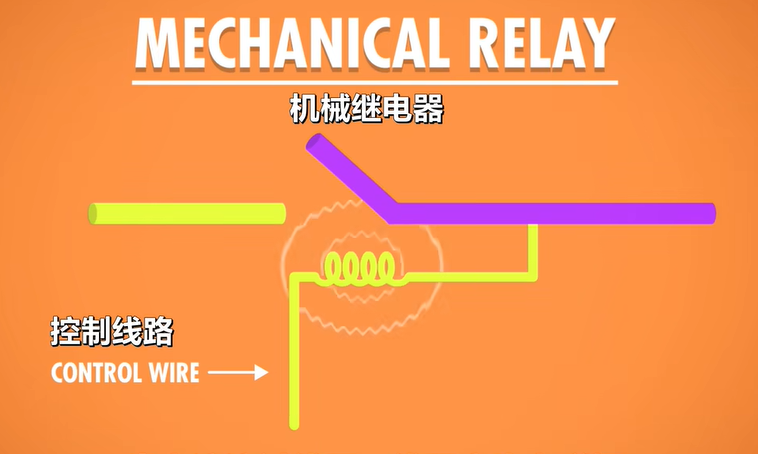
     • a control wire ：determines whether a circuit（电路；线路） is opened or closed

     • The control wire connects to a coil of wire inside the relay. When current flows through the coil, an electromagnetic field is created, which in turn, attracts a metal arm inside the relay， snapping it shut and completing the circuit. Relays control the electronics. The controlled circuit can then connect to other circuits, or to something like a motor(马达), which might increase a count on a gear(让计数齿轮+1), like in Hollerith’s tabulating machine就像iHollerith的制表机一样).

       coil /kɔɪl/ N-COUNT (绳子、金属丝等绕成的)卷，圈。 a coil of wire 一圈金属线

       current N-COUNT 电流

       electromagnetic /ɪˌlektrəʊmæɡˈnetɪk/ ADJ 电磁能的;电磁效应的

       electromagnetic field 电磁场

       in turn

       • 依次；轮流；逐个
         • The children called out their names in turn. 孩子们逐一自报姓名。
       • 相应地；转而 as a result of sth in a series of events 用于说明一种因果关系，表明接下来发生的事情是由前面的事情引发的
         • Increased production will, in turn, lead to increased profits. 增加生产会继而增加利润。

       snap /snæp/

       • [usually + 副词/介词短语] （使啪地）打开，关上，移到某位置 to move, or to move sth, into a particular position quickly, especially with a sudden sharp noise
         • [动词+形容词] The lid snapped shut. 盖子啪地合上了
         • His eyes snapped open. 他两眼唰地睁开了。
         • [单独使用的动词] He snapped to attention and saluted. 他啪一下立正敬礼。
         • [动词+名词短语+形容词] She snapped the bag shut.她啪的一声把包合上了。
       • (informal)拍照；摄影 to take a photograph

       shut /ʃʌt/

       • verb [I or T] (CLOSE) to (cause to) close something （使）关闭
       • verb [I or T] (STOP OPERATING) to (cause to) stop operating or being in service, either temporarily or permanently （使）停止运转;（使）停止营业
       • adjective [ after verb ] closed 关闭的，关上的

       completing the circuit 闭合电路

   • because the mechanical arm inside of a relay has mass, and therefore can’t move instantly between opened and closed states. As a result, computation speed is not fast.

   • the probability of a failure increases

   • relay has too short operational life（使用寿命)

   • attract insects (computer bug)

   • the Harvard Mark l

     • one of the largest
     • completed in 1944 by lBM for the Allies during World War 2
     • extremely large

2. vacuum tube.(真空管) /ˈvækjuːm/ /tjuːb/

   • thermionic valve（热电子管）

     • the first vacuum tube

     • In 1904, English physicist John Ambrose Fleming（约翰·安布罗斯·弗莱明)

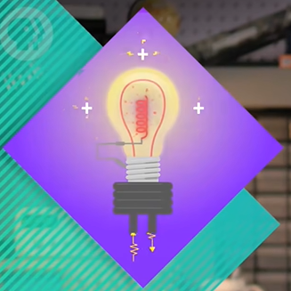
     • which housed（VERB 安置;容纳） two electrodes（电极） inside an airtight(密封的) glass bulb(电灯泡). One of the electrodes could be heated, which would cause it to emit electrons. The other electrode could then attract these electrons to create the flow of our electric(电的) faucet(水龙头), but only if(conj.只有；只有当) it was positively charged(带正电的).

       

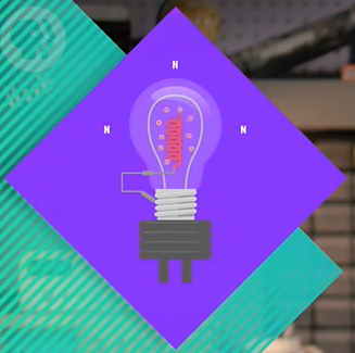
     • if it had a negative or neutral charge, the electrons would no longer be attracted across the vacuum, so no current would flow.

       

     • An electronic component that permits the one-way flow of current is called a diode（二极管）

   • triode vacuum tubes(三极真空管)

     • in 1906, American inventor Lee de Forest（李·德富雷斯特）

     • added a third “control” electrode that sits between the two electrodes. By applying a positive charge to the control electrode, it would permit the flow of electrons as before.

       

     • But if the control electrode was given a negative charge, it would prevent the flow of electrons.

       

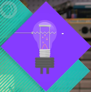
     • So by manipulating the control wire, one could open or close the circuit. lt’s pretty much the same thing as a relay.

     • expensive

     • 1940s, governments can afford

     • This marked the shift from electro-mechanical computing to electronic computing.

3. the transistor(晶体管)

   • In 1947 Bell Laboratory

   • The physics behind transistors is pretty complex, relying on quantum mechanics(量子力学)

   • A transistor is just like a relay or vacuum tube. it’s a switch that can be opened or closed by applying electrical power via a control wire. Typically, transistors have two electrodes separated by a material that sometimes can conduct electricity and other times resist it. This material called a semiconductor(半导体).

     

   • In this case,the control wire attaches to a “gate” electrode. By changing the electrical charge of the gate, the conductivity of the semiconducting material can be manipulated, allowing current to flow or be stopped

     

   • transistors were solid material

   • This led to dramatically smaller and cheaper computers, like the IBM 608, released in 1957

   • Today, computers use transistors that are smaller than 50 nanometers in size – for reference,a sheet of paper is roughly 100,000 nanometers thick.

   • Silicon Valley

   • Shockley Semiconductor —> Fairchild Semiconductors —> Intel

Boolean Logic & Logic Gates

1. Binary(二进制)

   • representing the values “true” and “false”

     • In computers, an “on” state when electricity is flowing, represents true. The off state, no electricity flowing, represents false. We can also write binary as 1‘s and 0’s instead of true’s and false’s

   • The reason of use Binary

     • the more intermediate states there are, the harder it is to keep them all separate
     • an entire branch of mathematics already existed that dealt exclusively with true and false values. It’s called Boolean Algebra(布尔代数)!

2. three fundamental operations in Boolean Algebra: a NOT, an AND, and an OR operation.

   • You can think of the control wire as an input, and the wire coming from the bottom electrode as the output. So with a single transistor, we have one input and one output.

     

   • If we turn the input on, the output is also on because the current can flow through it. If we turn the input off, the output is also off and the current can no longer pass through.

     

   • a logic table(真值表)：can’t doing any thing

     

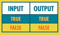
3. Not Gate

   • Instead of having the output wire at the end of the transistor we can move it before. If we turn the input on, the transistor allows current to pass through it to the “ground”, and the output wire won’t receive that current, so it will be off. In our water metaphor(比喻) grounding would be like if all the water in your house was flowing out of a huge hose, so there wasn’t any water pressure left for your shower. So in this case if the input is on, output is off. When we turn off the transistor though, current is prevented from flowing down it to the ground, so instead, current flows through the output wire.

     

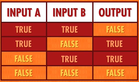
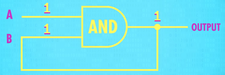
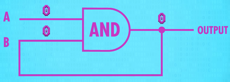
4. And Gate

   To build an AND gate, we need two transistors connected together so we have our two inputs and one output. If we turn on just transistor A current won’t flow because the current is stopped by transistor B. Alternatively if transistor B is on, but the transistor A is off, the same thing, the current cant get through. Only if transistor A AND transistor B are on does the output wire have current.

   

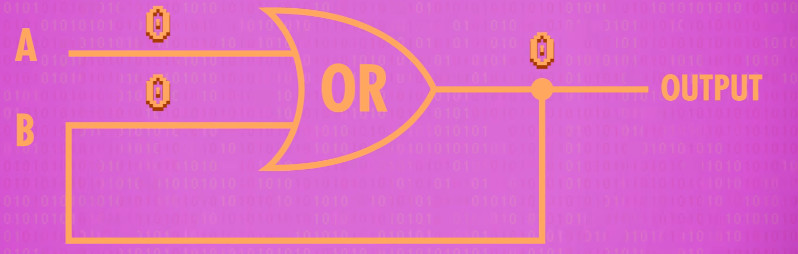
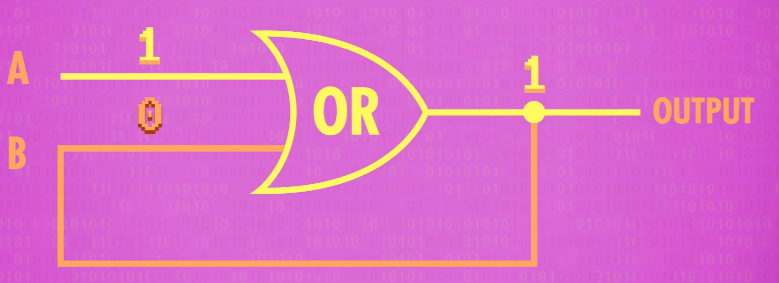
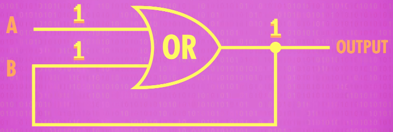
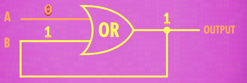
5. Or Gate

   Building an OR gate from transistors needs a few extra wires. Instead of having two transistors in series(串联) – one after the other – we have them in parallel(并联). We run wires from the current source to both transistors. We use this little arc to note that the wires jump over one another and aren’t connected,even though they look like they cross. If both transistors are turned off the current is prevented from flowing to the output, so the output is also off. Now, if we turn on just Transistor A, current can flow to the output. Same thing if transistor A is off, but Transistor B in on. Basically if A OR B is on, the output is also on. Also, if both transistors are on, the output is still on.

   

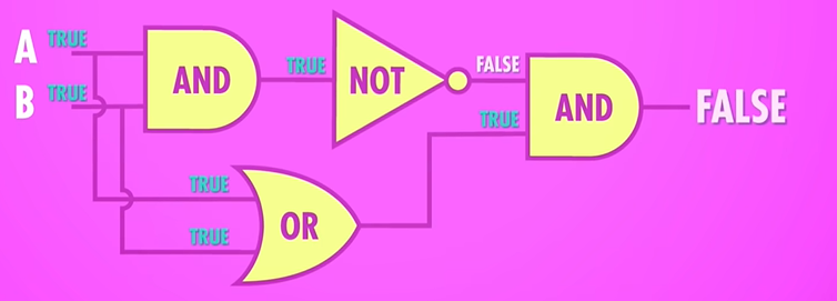
6. abstraction of Not&And&Or

   • Not：a triangle with a dot

     

   • And: D

     

   • Or: spaceship

     

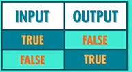
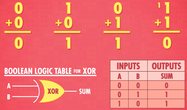
7. Exclusive OR = XOR（异或）

   • XOR is like a regular OR, but with one differences：if both inputs are true, the XOR is false. It is like when you go out to dinner and your meal comes with a side salad OR a soup. you can’t have both!

     

   • And building this(XOR) from transistors is pretty confusing, but we can show how an XOR is created from our three basic boolean gates.

     

   • XOR: an OR gate with a smile

     

Representing Numbers and Letters with Binary

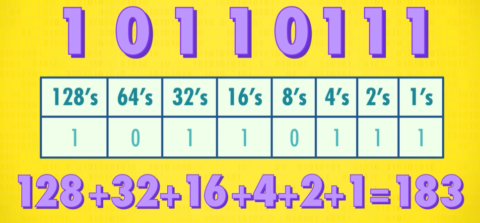
1. Instead of true and false,we can call these two states 1 and 0.

2. Take for example the binary number 101. This means we have 1 four, 0 twos, and 1 one. Add those all together and we’ve got the number 5 in base ten.

   

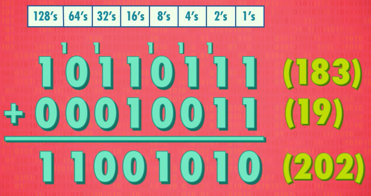
3. Binary addition

   

4. Each of these binary digits, 1 or 0, is called a “bit“(位)。

5. So in these last few examples, we were using 8-bit numbers with their lowest value of zero and highest value is 255, which requires all 8 bits to be set 1.

6. And 8-bits is such a common size in computing, it has a special word: a byte(字节).

7. 1 bytes=8 bits

8. two conversion method：

   • International System of Units：
     • 1 kilobyte（KB） = 1 thousand bytes
     • Mega is a million bytes (MB)
     • giga is a billion bytes (GB)
     • 1 terabyte is a trillion bytes (TB)
   • more common in computer ： 1 KB = 2^10^ bytes = 1024 B

9. 32-bit or 64-bit computers：What this means is that they operate in chunks of 32 or 64 bits.

10. positive and negative numbers：

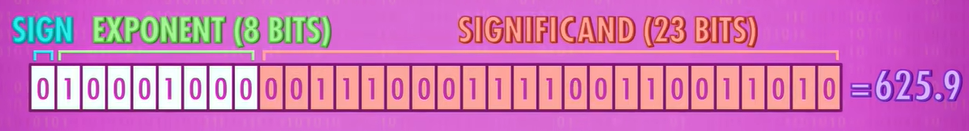
    • Most computers use the first bit for the sign：1 for negative, 0 for positive numbers,

11. not whole numbers(非整数) OR “floating point” numbers(浮点数)：

    • IEEE 754 standard：625.9 can be written as 0.6259 X 10^3^

      • the .6259 is called the significand(有效数)

      • 32-bit floating point number：625.9

        

12. computers simply use numbers to represent letters：number(VERB 把…编号) the letters of the alphabet

13. ASCII : the American Standard Code for Information Interchange 美国信息交换标准代码

    • Invented in 1963, ASCII was a 7-bit code, enough to store 128 different values

    • it did have a major limitation: it was really only designed for English

    • Fortunately, there are 8 bits in a byte, not 7, and it soon became popular to use codes 128 through 255, previously unused, for “national” characters. Different countries used these extra codes to encode their own characters.

      • if you opened an email written in Latvian on a Turkish computer,the result was completely incomprehensible. （scrambled text(乱码))
      • Chinese and Japanese have thousands of characters. There was no way to encode all those characters in 8- bits.

14. Unicode

    • devised(VERB 设计;发明;策划;想出) in 1992
    • it replaced them with one universal encoding scheme
    • The most common version of Unicode uses 16 bits with space for over a million codes
    • other file formats - like MP3s or GlFs - use binary numbers to encode sounds or colors of a pixel(N-COUNT 像素) in our photos, movies, and music.

How Computers Calculate

1. Arithmetic and Logic Unit – ALU – 算术逻辑单元

2. the Intel 74181:

   • the most famous ALU ever
   • it was released in 1970
   • the first complete ALU that fit entirely inside of a single chip(芯片)
   • the 74181 could only handle 4-bit inputs

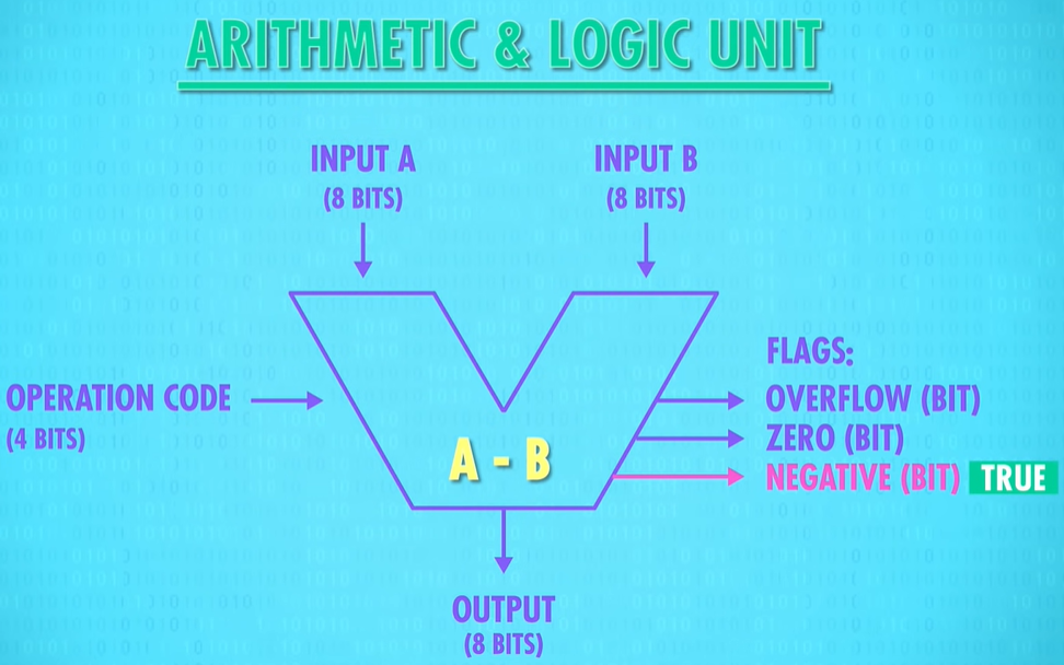
3. An ALU is really two units in one – there’s an arithmetic unit and a logic unit

4. arithmetic unit：is responsible for handling all numerical operations in a computer

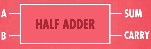
   • So we have two inputs, A and B, and one output, which is the sum of those two digits. A, B and the output are all single bits (0 or 1).

     

   • carry bit 进位：we need an extra output wire for that carry bit. The carry bit is only “true” when the inputs are 1 AND 1, because that’s the only time when the result (two)is bigger than 1 bit can store and conveniently we have a gate for that! An AND gate, which is only true when both inputs are true, So well add that to our circuit too.

     

   • This circuit is called a half adder (半加器)

     

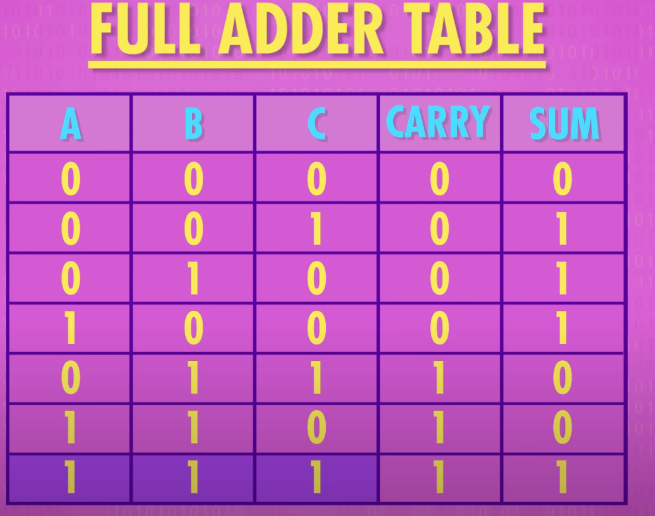
   • Full adder(全加速器)：

     • If you want to add more than 1+ 1 we’re going to need a “Full Adder”. That half-adder left us with a carry bit as output. That means that when we move on to the next column in a multi-column addition, and every column after that, we are going to have to add three bits together, no two.

       

     • A full adder is a bit more complicated - it takes three bits as inputs: A B and C. So the maximum possible input is 1+1+1, which equals 1 carry out 1(等于1并且进一位), so we still only need two output wires sum and carry

       

     • building a full adder：

       
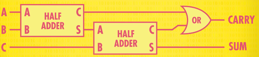
       • we need a OR gate to check if either one of the carry bits was true

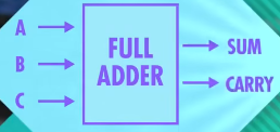
     • abstraction of full adder :

       

   • BUILDING AN 8-BIT ADDER（8位加法器)

     

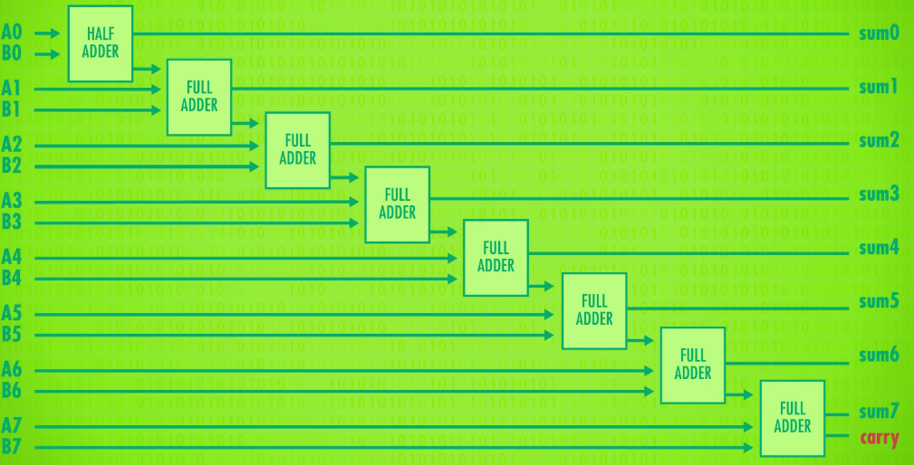
     Notice that our last full adder has a carry out(进位输出). If there is a carry into the 9th bit, it means the sum of the two numbers is too large to fit into 8-bits. This is called an overflow（溢出）. In general, an overflow occurs when the result of an addition is too large to be represented by the number of bits you are using. This can usually cause errors and unexpected behavior. So if we want to avoid overflows, we can extend our circuit with more full adders, allowing us to add 16 or 32 bit numbers. This makes overflows less likely to happen, but at the expense of more gates. An additional downside is that it takes a little bit of time for each of the carries to ripple forward. Admittedly, not very much time, electrons move pretty fast, so we’re talking about billionths of a second, but that’s enough to make a difference in today’s fast computers. For this reason, modern computers use a slightly different adding circuit called a carry-look-ahead adder（超前进位加法器) ，which is faster, but ultimately does exactly the same thing – adds binary numbers.

     ripple /ˈrɪpl/ [动词+ 副词/介词短语] of a feeling, etc. 感觉等扩散；涌起 to spread through a person or a group of people like a wave。“ripple” 的意思是像涟漪一样扩散、传播、波动，在这里用于形象地描述进位（carries）逐步向前传递的过程，就像水波泛起涟漪一样，一个接着一个地向前推进，强调进位的传递是有一个过程且是逐步进行的

     billionth /ˈbɪljənθ/ FRACTION 十亿分之一 。 a billionth of a second 十亿分之一秒

   • there are no multiply and divide operations in ALU. That’s because simple ALUs don’t have a circuit for this,and instead just perform a series of additions. Let’s say you want to multiply 12 by 5. That’s the same thing as adding 12 to itself 5 times.

   • However, fancier processors(更贵的/更好的处理器), like those in your laptop or smart phone, have arithmetic units(计算单元) with dedicated(专用的) circuits for multiplication(乘法).

5. the Logic Unit（逻辑单元）

   • Instead of arithmetic operations, the Logic Unit performs well logical operations, like AND, OR and NOT which we’ve talked about previously. It also performs simple numerical tests, like checking if an umber is negative.

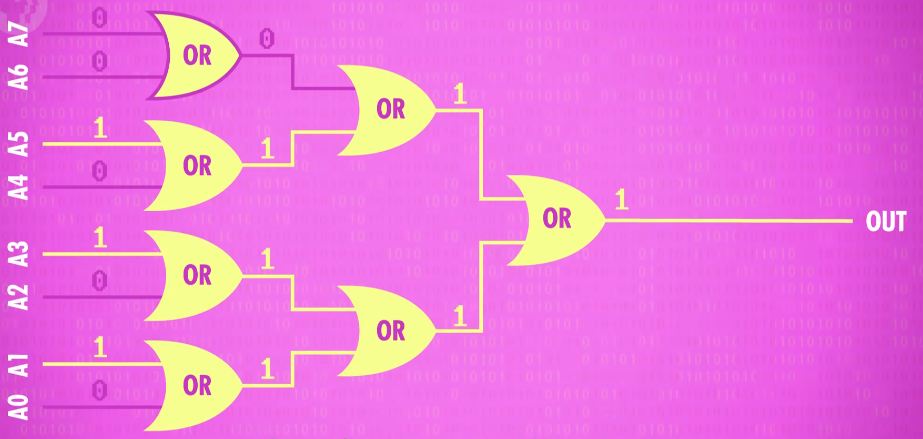
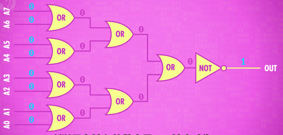
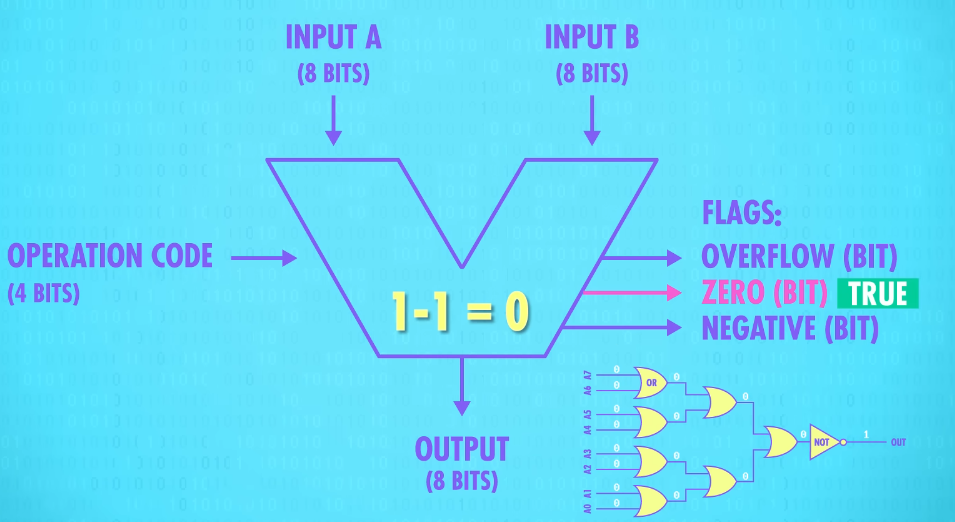
   • For example, here is a circuit that tests if the output of the ALU is zero. It does this using a bunch of OR gates to see if any of the bits are 1. Even if one single bit is 1, we know the number can’t be zero and then we use a final NOT gate to flip this input so the output is 1 only if the input number is 0.

     

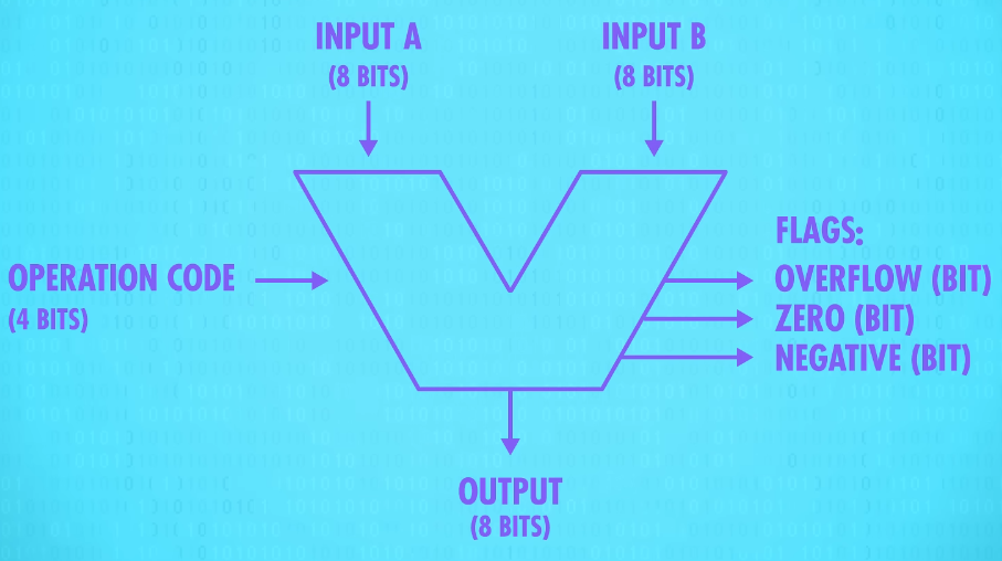
6. abstraction of ALU

   

7. Our 8-bit ALU has two inputs, A and B, each with 8 bits. We also need a way to specify(VERB 明确说明;具体指定) what operation the ALU should perform, for example, addition or subtraction. For that, we use a 4-bit operation code. We’ll talk about this more in a later episode, but in brief, 1000 might be the command to add, while 1100 is the command for subtract.

   

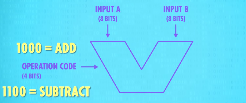
   Basically, the operation code tells the ALU what operation to perform. And the result of that operation on inputs A and B is an 8-bit output. ALUs also output a series of Flags, which are 1-bit outputs for particular states and statuses.

   

   For example, if we subtract two numbers, and the result is 0, our zero-testing circuit the one we made earlier, sets the Zero Flag to True(1). This is useful if we are trying to determine if two numbers are equal.

   

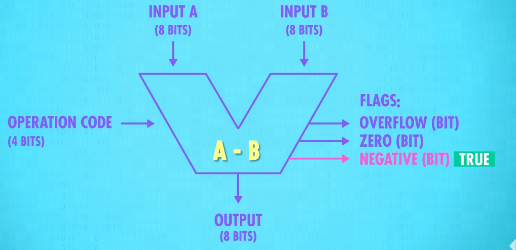
   If we wanted to test if A was less than B, we can use the ALU to calculate A subtract B and look to see if the Negative Flag was set to true(1). If it was, we know that A was smaller than B.

   

   And finally, there’s also a wire attached to the carry-out on the adder we built, so if there is an overflow we’ll know about it. This is called the Overflow Flag.

   “carry-out” 指的是加法运算中产生的进位输出信号或结果

Registers and RAM

1. Random Access Memory：RAM（随机存取存储器）

   • stores things like game state- as long as the power stays on.

2. persistent memory（持久存储）：can survive without power

3. Gated Latch（锁存器）

   • Let’s try taking an ordinary OR gate, and feed the output back into one of its inputs. First, let’s set both inputs to 0. So 0 OR 0 is 0 and so this circuit always outputs 0.

     

     If we were to flip input A to 1. 1 OR 0 is 1, so now the output of the OR gate is 1.

     

     A fraction of a second later, that loops back around into input B, so the OR gate sees that both of its inputs are now 1. 1 OR 1 is still 1, so there is no change in output.

     

     If we flip input A back to 0, the OR gate still outputs 1. So now we’ve got a circuit that records a “1” for us.

     

     Except, we’ve got a teensy(很小的) tiny problem-this change is permanent! No matter how hard we try there’s noway to get this circuit to flip back from a 1 to a 0.

   • Now lets look at this same circuit but with an AND gate instead. We’ll start inputs A and B both at 1. 1 AND 1 outputs 1 forever.

     

     But if we then flip input A to 0, because it’s an AND gate, the output will go to 0.

     

     So this circuit records a 0, the opposite of our other circuit. Like before**, no matter what input we apply to input A afterwards, the circuit will always output 0**.

   • AND-OR Latch（AND-OR 锁存器）

     It has two inputs, a “set” input, which sets the output to a 1, and a “reset” input, which resets the output to a 0.

     

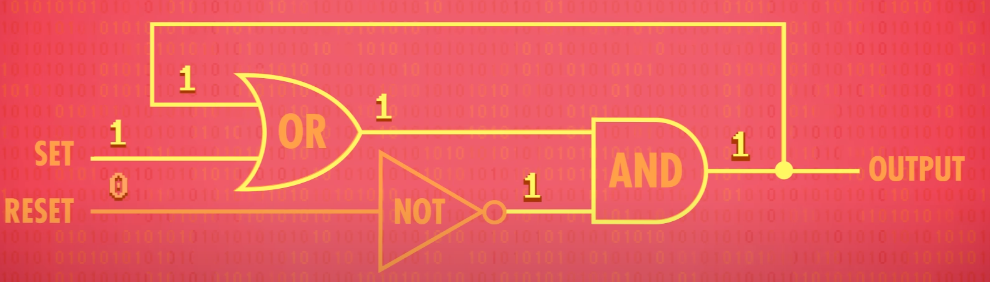
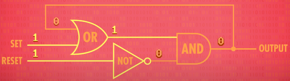
     If set and reset are both 0, the circuit just outputs whatever was last put in it. In other words, it remembers a single bit of information!

     

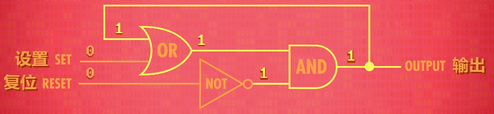
     This is called a “latch” because it “latches onto” a particular value and stays that way. The action of putting data into memory is called writing, whereas getting the data out is called reading.

   • Gated Latch（锁存器）

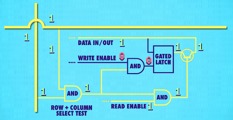
     To make this a little easier to use, we really want a single wire to input data that we can set to either 0 or 1 to store the value. Additionally, we are going to need a wire that enables the memory to be either available for writing or locked down - which is called the write enable line.

     

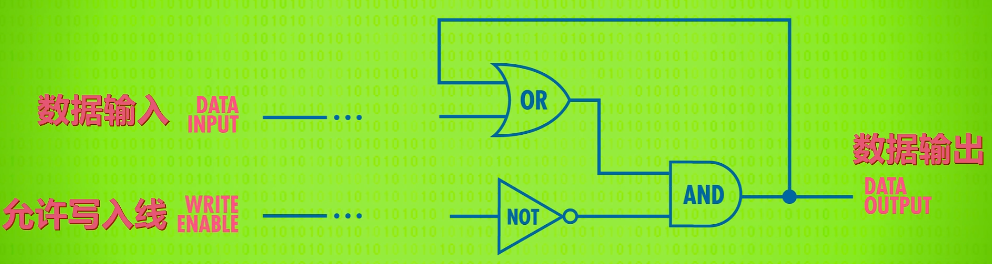
     By adding a few extra logic gates, we can build this circuit, which is called a Gated Latch since the gate can be opened or closed.

     

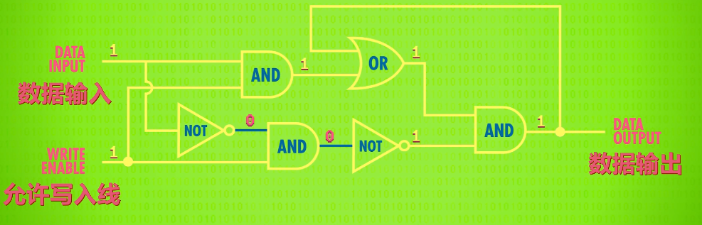
   • abstraction ：put our whole Gated Latch circuit in a box – a box that stores one bit.

     

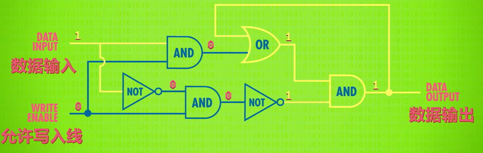
     If we toggle the Data wire from 0 to 1 or 1 to 0, nothing happens-the output stays at 0. That’s because the write enable wire is off which prevents any change to the memory.

     

     So we need to “open” the “gate” by turning the write enable wire to 1. Now we can put a 1 on the data line to save the value 1 to our latch.

     

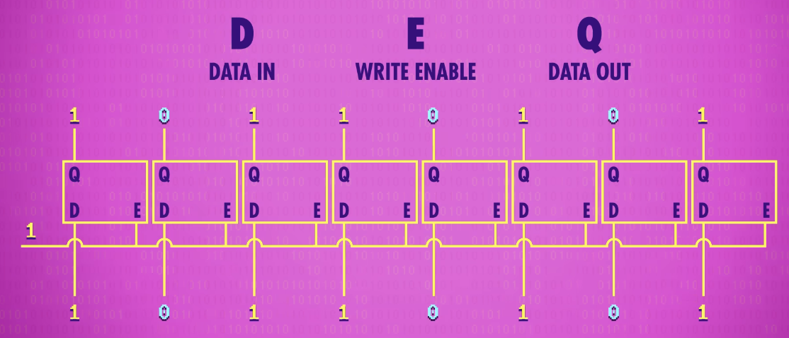
4. Register(寄存器)

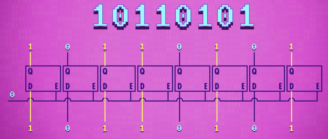
   • If we put 8 latches side-by-side, we can store 8 bits of information like an 8 bit number. A group of latches operating like this is called a register, which holds a single number and the number of bits(位数) in a register is called its width(位宽),

   • Early computers had 8-bit registers, then 16, 32, and today, many computers have registers that are 64-bits wide.

   • To write to our register, we first have to enable all of the latches. We can do this with a single wire that connects to all of their enable inputs, which we set to 1. We then send our data in using the 8 data wires, and then set enable back to 0, and the 8 bit value is now saved in memory.

     

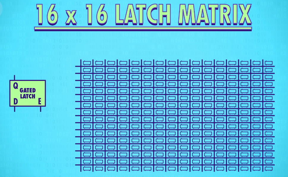
5. For 256-bit register, we end up with 513(256+256+1) wires! The solution is a matrix(矩阵)! In this matrix we don’t arrange our latches in a row, we put them in a grid(网格). For 256 bits, we need a 16 by 16 grid of latches with 16 rows and columns of wires.

   

   To activate any one latch, we must turn on the corresponding(相关的) row AND column wire.

   

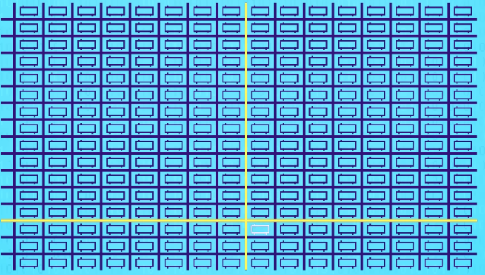
   Let‘s zoom in and see how this works. We only want the latch at the intersection of the two active wires(两根active wires交叉处的锁存器) to be enabled, but all of the other latches should stay disabled. For this, we can use our trusty(可靠的) AND gate. The AND gate will output a only if the row and the column wires are both 1. So we can use this signal(信号-two active wires) to uniquely select a single latch.

   zoom in /zuːm ɪn/ ：VERB （摄像机或摄影机）拉近镜头，进行近景拍摄 (~ on sth)

   

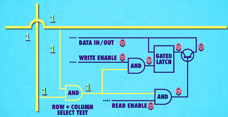
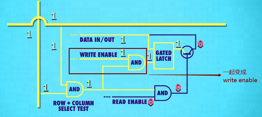
   This row/column set-up connects all our latches with a single,shared write enable wire(允许写入线).

   set-up ： N-SING (软件或硬件的)安装，设置

   翻译：这种行/列排列法，用一根”允许写入线”连所有锁存器

   

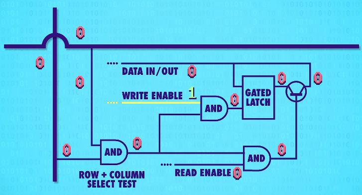
   In order for a latch to become write enabled, the row wire, the column wire, and the write enable wire must all be 1.

   

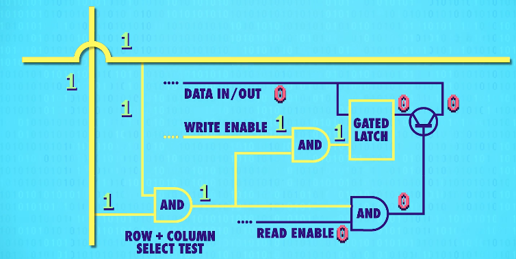
   That should only ever be true for one single latch at any given time. This means we can use a single, shared wire for data. Because only one latch will ever be write enabled, only one will ever save the data – the rest of the latches will simply ignore values on the data wire because they are not write enabled.

   

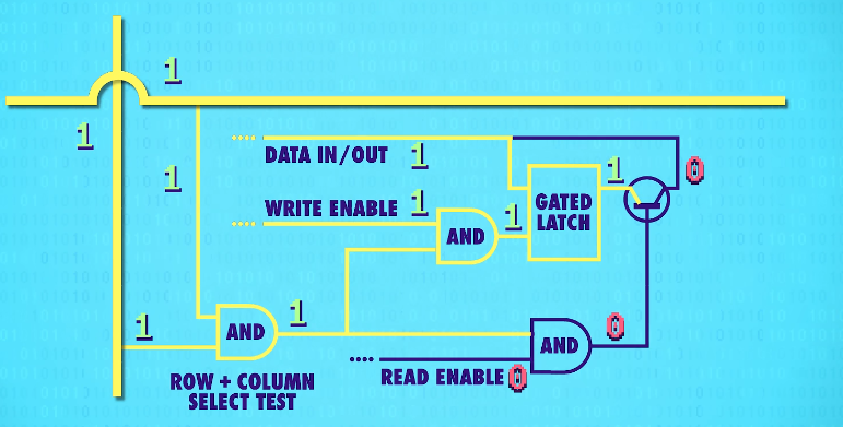
   We can use the same trick with a read enable wire to read the data later, to get the data out of one specific latch.

   

   This means in total, for 256 bits of memory, we only need 35 wires – 1 data wire,1 write enable wire, 1 read enable wire, and 16 rows and columns(16根行线+16根列线) for the selection.

6. memory address：存储器地址；内存地址

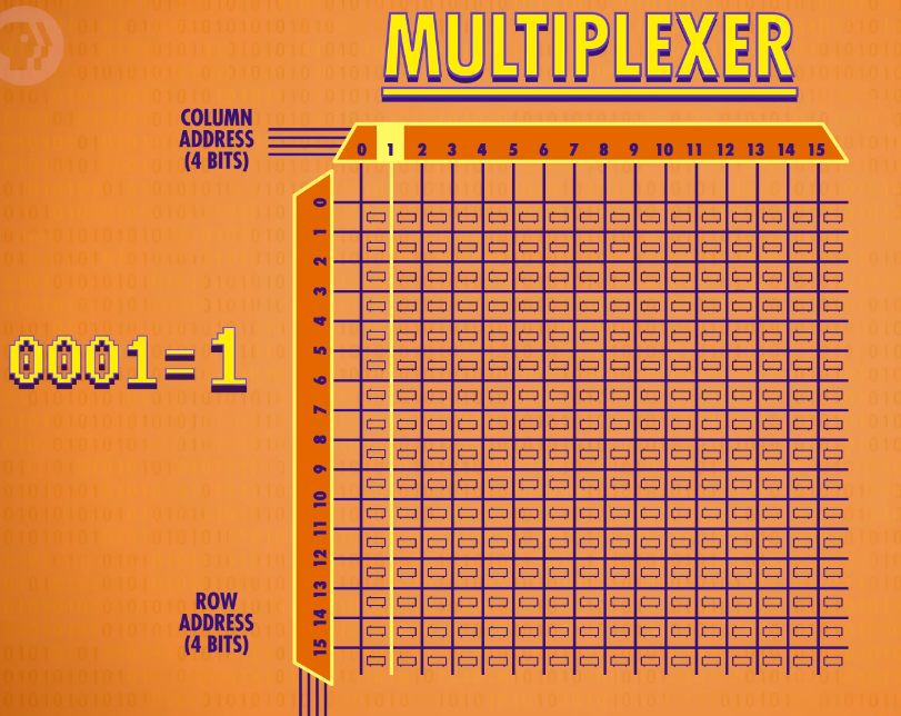
   The latch we just saved our one bit into has an address of row 12 and column 8. Since there is a maximum of 16 rows, we store the row address in a 4 bit number. 12 is 1100 in binary. We can do the same for the column address: 8 is 1000 in binary. So the address for the particular latch we just used can be written as 11001000.

7. multiplexer(多路复用器)：convert from an address into something that selects the right row or column

   Multiplexers come in all different sizes, but because we have 16 rows, we need a 1 to 16 multiplexer. It works like this. You feed it a 4 bit number, and it connects the input line to a corresponding output line. So if we pass in 0000, it will select the very first column for us. If we pass in 0001 the next column is selected, and so on. We need one multiplexer to handle our rows and another multiplexer to handle the columns.

   

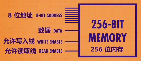
8. abstraction of 256-bit memory： It takes an 8-bit address for input - the 4 bits for the column and 4 for the row. We also need write and read enable wires. And finally, we need just one data wire, which can be used to read or write data.

   

9. Unfortunately. even 256-bits of memory isn’t enough to run much of anything, so we need to scale up even more! We’re going to put them in a row. Just like with the registers. We’ll make a row of 8 of them, so we can store an 8 bit number - also known as a byte. To do this, we feed the exact same address into all 8 of our 256-bit memory components at the same time, and each one saves one bit of the number. That means the component we just made can store 256 bytes at 256 different addresses.

   

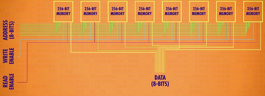
10. abstraction of RAM : we’ll think of it as a uniform bank of addressable memory. We have 256 addresses, and at each address, we can read or write an 8-bit value.

    addressable memory：可寻址的内存

    在计算机领域，“bank” 常见释义为 “存储体；存储库”

    

11. The way that modern computers scale to megabytes and gigabytes of memory is by doing the same thing we’ve been doing here – keep packaging up little bundles of memory into larger, and larger, and larger arrangements. As the number of memory locations grow,our addresses have to grow as well. 8 bits hold enough numbers to provide addresses for 256 bytes of our memory, but that’s all. To address a gigabyte– or a billion bytes of memory – we need 32-bit addresses.

    scale /skeɪl/ (technical 术语)改变…的大小; 扩大规模；扩展 to change the size of sth

    gigabyte /ˈɡɪɡəbaɪt/ 千兆字节(GB)

12. An important property of this memory is that we can access any memory location, at any time, and in a random order. For this reason, it’s called Random-Access Memory or RAM.

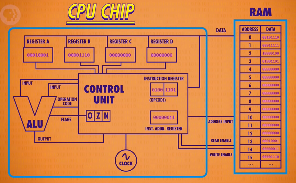
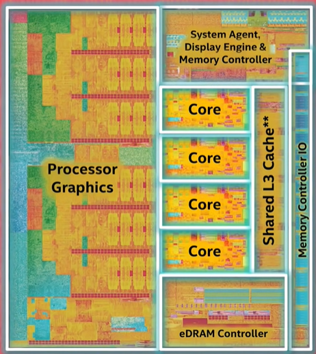
The Central Processing Unit (CPU)

1. the Central Processing Unit（中央处理单元），CPU

2. build up a simple CUP

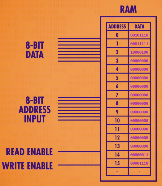
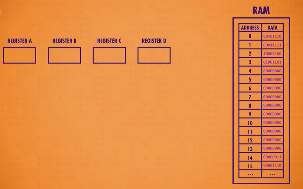
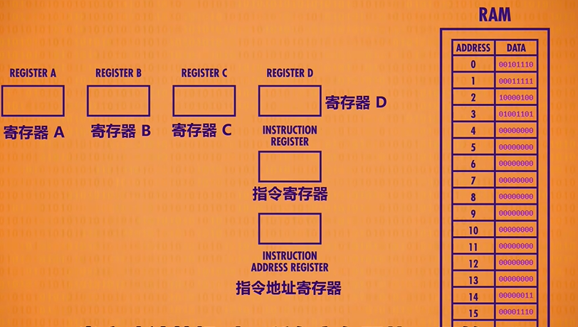
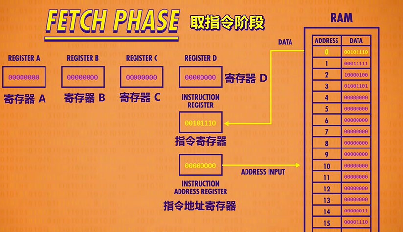
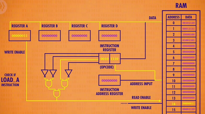
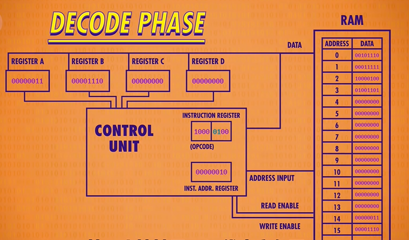
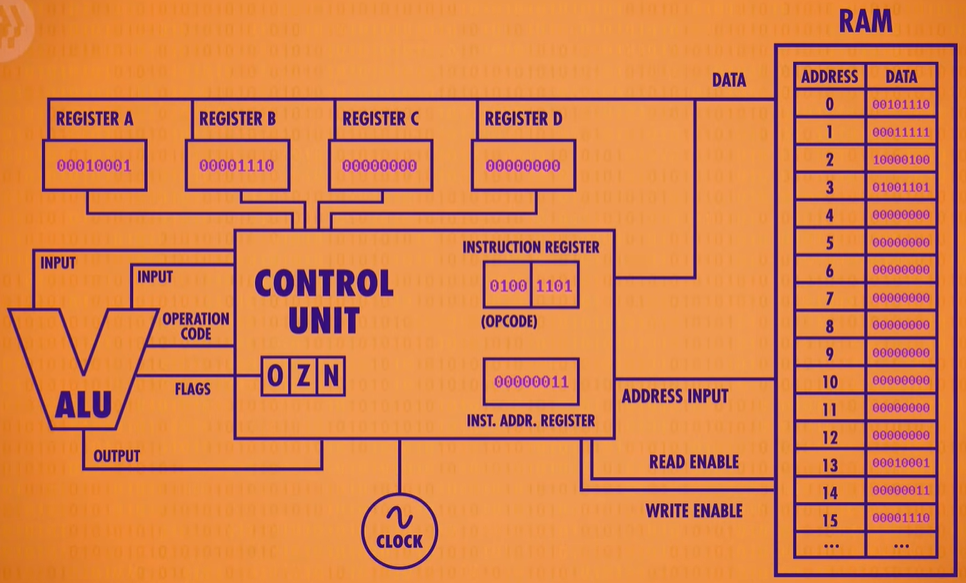
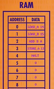
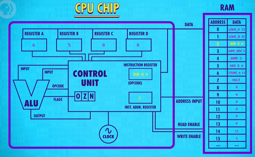
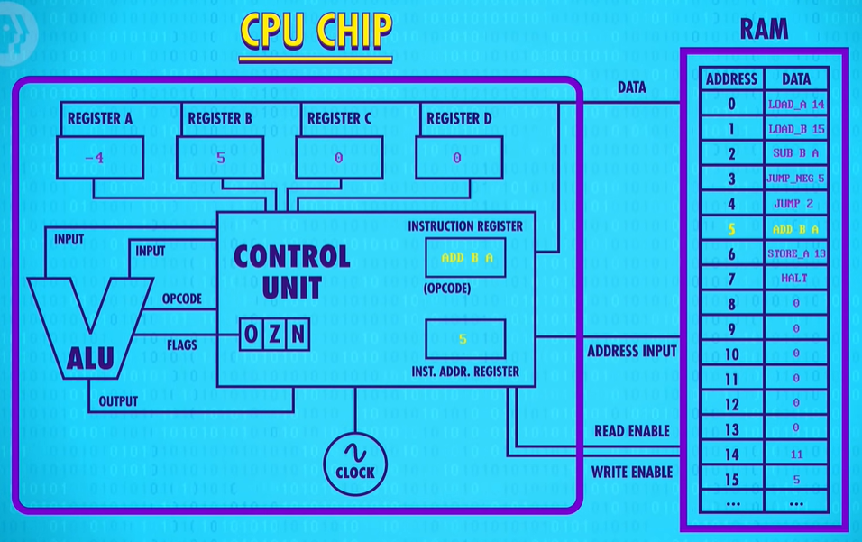
   • Let’s drop in the RAM module we created last episode. To keep things simple, we’ll assume it only has 16 memory locations, each containing 8 bits. Let’s also give our processor four 8-bit memory registers, labeled A B C and D which will be used to temporarily store and manipulate values.

     

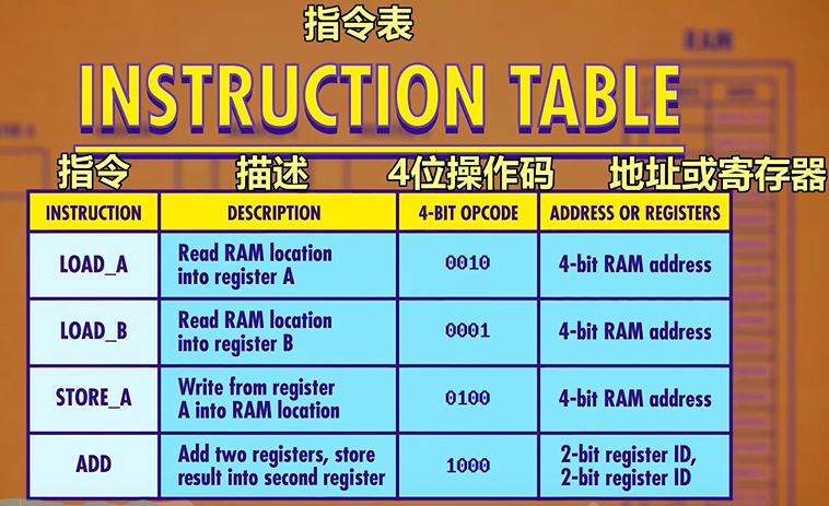
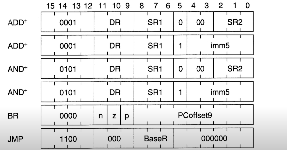
   • We already know that data can be stored in memory as binary values and programs can be stored in memory too. We can assign an ID to each instruction supported by our CPU. In our hypothetical example, we use the first four bits to store the “operation code”, or opcode for short. The final four bits specify where the data for that operation should come from - this could be registers or an address in memory.

     

   • We also need two more registers to complete our CPU. First we need a register to keep track of where we are in a program. For this, we use an instruction address register, which as the name suggests, stores the memory address of the current instruction. And then we need the other register to store the current instruction, which we’ll call the instruction register.

     

3. LOAD A : Read RAM location into register A

   • When we first boot up our computer all of our registers start at 0. As an example, we’ve initialized our RAM with a simple computer program that we’ll to through today. The first phase of a CPU’s operation is called the fetch phase（取指令阶段）. This is where we retrieve our first instruction. First, we wire our Instruction Address Register to our RAM module. The register’s value is 0, so the RAM returns whatever value is stored in address 0. In this case, 00101110. Then this value is copied in to our instruction register.

     

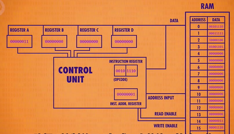
   • Now that we’ve fetched an instruction from memory, we need to figure out what that instruction is so we can execute it. This is called the decode phase（解码阶段）. In this case the opcode, which is the first four bits, is : 0010. This opcode corresponds to the “LOAD A” instruction, which loads a value from RAM into Register A. The RAM address is the last four bits of our instruction which are 1110 or 14 in decimal.

     

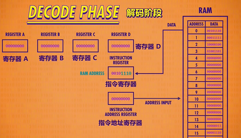
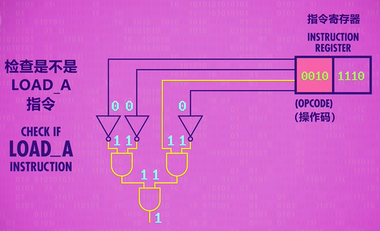
   • Next instructions are decoded and interpreted by a Control Unit（单元控制）. Like everything else we’ve built, it too is made out of logic gates. For example, to recognize a LOAD A instruction, we need a circuit that checks if the opcode matches 0010, which we can do with a handful of logic gates.

     

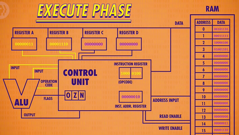
   • Now that we know what instruction we’re dealing with, we can go ahead and perform that instruction which is the beginning of the execute phase（执行阶段）! Using the output of our LOAD A checking circuit, we can turn on the RAM’s read enable line and send in address 14（1110）. The RAM retrieves the value at that address, which it 00000011 or 3 in decimal.

     

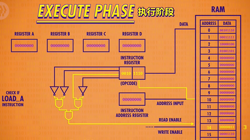
   • Now because this is a LOAD A instruction, we want that value to only be saved into Register A and not any of the other registers. So if we connect the RAM’s data wires to our four data registers, we can use our LOAD A check circuit（检查是否LOAD A 的线路） to enable the write enable（允许写入线） only for Register A. We’ve successfully loaded the value at RAM address 14 into Register A.

     

   • We’ve completed the instruction, so we can turn all of our wires off, and we are ready to fetch the next instruction in memory. To do this, we increment the Instruction Address Register by 1 which completes the execute phase.

     

   • LOAD A is just one of several possible instructions that our CPU can execute. Different instructions are decoded by different logic circuits, which configure the CPU’s components to perform that action.

   • Looking at all those individual decode circuits is too much detail, so since we looked at one example, we’re going to go head and package them all up as a single Control Unit to keep things simple.

     

4. LOAD B : Read RAM location into register B

   • Having completed one full fetch/decode/execute cycle, we’re ready to start all over again, beginning with the fetch phase. The Instruction Address Register now has the value 1 in it, so the RAM gives us the value stored at address 1, which is 0001 111.

     

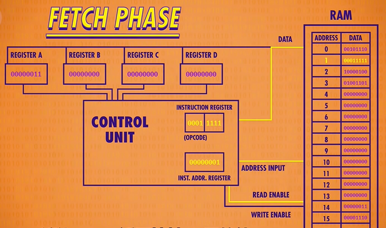
   • On to the decode phase! 0001 is the “LOAD B” instruction, which moves a value from RAM into Register B. The memory location this time is 1111 which is 15 in decimal.

   • Now to the execute phase! The Control Unit configures the RAM to read address 15 and configures Register B to receive the data. Bingo, we just saved the value 00001110 or the number 14 in decimal into Register B.

     

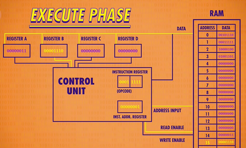
   • Last thing to do is increment our instruction address register by 1, and we’re done with another cycle.

5. ADD : Add two registers, store result into second register

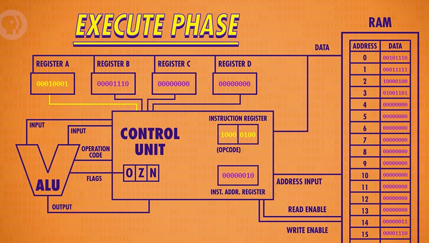
   • That opcode 1000 is an ADD instruction. Instead of an 4-bit RAM address, this instruction uses two sets of 2 bits. Remember that 2 bits can encode 4 values, so 2 bits is enough to select anyone of our 4 registers. The first set of 2 bits is 01, which in this case corresponds to Register B, and 00, which is Register A. So “1000 01 00” is the instruction for adding the value in Register B into the value in register A.

     

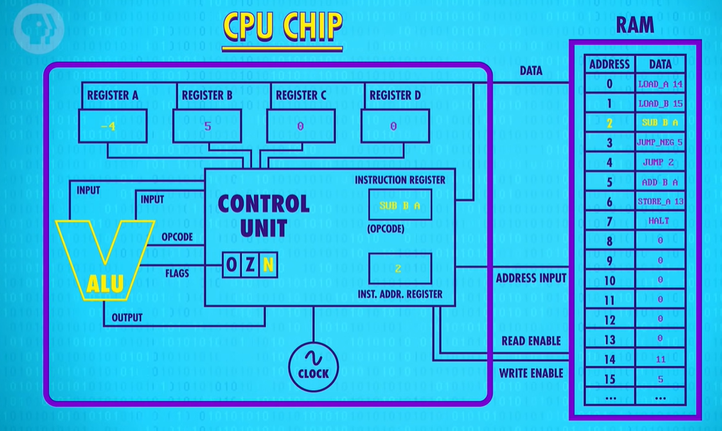
   • So to execute this instruction, we need to integrate the ALU into our CPU. The Control Unit is responsible for selecting the right registers to pass in as inputs, and configuring the ALU to perform the right operation. For this ADD instruction the Control Unit enables Register B and feeds its value into the first input of the ALU. It also enables Register A and feeds it into the second ALU input. As we already discussed, the ALU itself can perform several different operations, so the Control Unit must configure it to perform an ADD operation by passing in the ADD opcode.

     

   • Finally the output should be saved into Register A. But it can’t be written directly, because the new value would ripple back into the ALU and then keep adding to itself. So the Control Unit uses an internal register to temporarily save the output, turn off the ALU, and then write the value into the proper destination register. In this case, our inputs were 3 and 14 and so the sum is 17 or 00010001 in binary, which is now sitting in Register A.

     

   • As before, the last thing to do is increment our instruction address by 1.

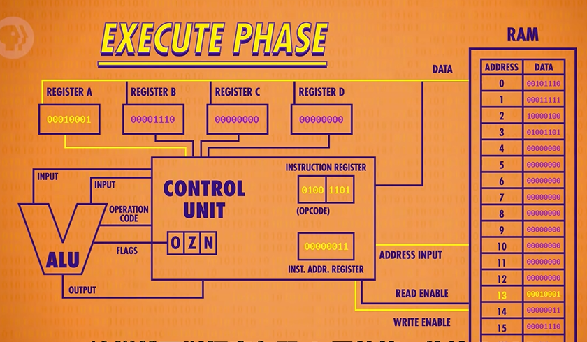
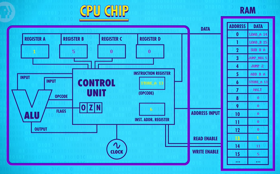
6. STORE A : Write from register A into RAM location

   • When we decode it we see that 0100 is a STORE A instruction, with a RAM address of 13. As usual, we pass the address to the RAM module, but instead of read-enabling the memory we write-enable it. At the same time, we read-enable Register A. This allows us to use the data line to pass in the value store in register A.

     

7. Our first program: It loaded two values from memory, added them together, and then saved that sum back into memory.

8. Of course, by me talking you through the individual steps, I was manually transitioning the CPU through its fetch, decode and execute phases. So the responsibility of keeping the CPU ticking along falls to a component called the clock. As its name suggests, the clock triggers an electrical signal at a precise and regular interval. Its signal is used by the Control Unit to advance the internal operation of the CPU, keeping everything in lock-step. Of course you can’t go too fast, because even electricity takes some time to travel down wires and for the signal to settle. The speed at which a CPU can carry out each Step of the fetch-decode-execute cycle is called its Clock Speed(时钟速度). This speed is measured in Hertz(赫兹) - a unit of frequency. One Hertz means one cycle per second.

   

9. The very first single-chip CPU was the Intel 4004, a 4-bit CPU released in 1971. Despite being the first processor of its kind, it had a mind-blowing clock speed of 740 Kilohertz - that’s 740 thousand cycles per second.

10. One megahertz is one million clock cycles per second, and the computer or even phone that you are watching this video on right now is no doubt a few gigahertz(兆赫兹) - that’s billions of CPU cycles every single second.

11. abstraction Of CUP ：RAM lies outside the CPU as its own component, and they communicate with each other using address, data and enable wires.

    

Instructions & Programs

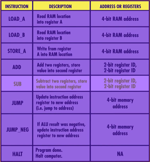
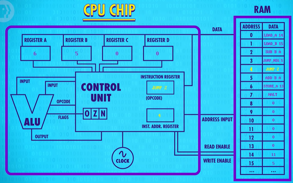
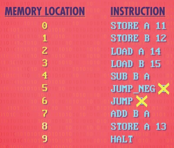
1. JUMP: Update instruction address register to new address. As the name implies, this causes the program to “jump” to a new location. This is useful if we want to change the order of instructions or choose to skip some instructions. For example, a JUMP 0, would cause the program to go back to the beginning. At a low level, this is done by writing the value specified in the last four bits into the instruction address register, overwriting the current value.

2. JUMP_NEGATIVE : This only jumps the program if the ALU’s negative flag is set to true. As we talked about in Episode 5, the negative flag is only set when the result of an arithmetic operation is negative. If the result of the arithmetic was zero or positive, the negative flag would not be set.

   

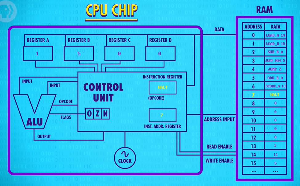
3. HALT : And finally computers need to be told when to stop processing, so we need a HALT instruction. Our previous program really should have a HALT instruction at end of program, otherwise the CPU would have just continued on after the STORE instruction, processing all those 0’s. But here is no instruction with an opcode of 0 and so the computer would have crashed ! It’s important to point out here that we’re storing both instructions and data in the same memory. So the HALT instruction is really important because it allows us to separate the two.

   

4. JUMP

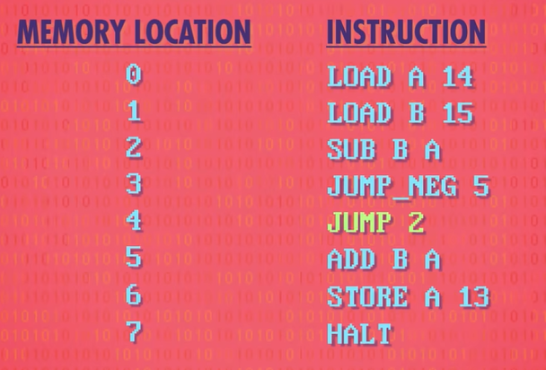
   First LOAD_A 14 loads the value 1 into Register A. Next, LOAD_B 15 loads the value 1 into Register B. As before, we ADD registers B and A together with the sum going into Register A. 1+1=2, so now Register A has the value 2 in it ( stored in binary of course ). Then the STORE instruction saves that into memory location 13.

   

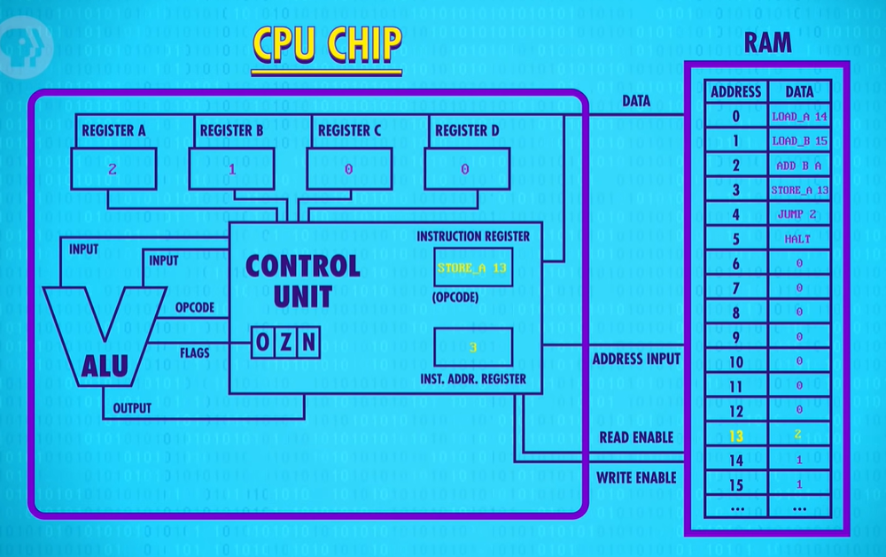
   Now we hit a “JUMP 2“ instruction.

   

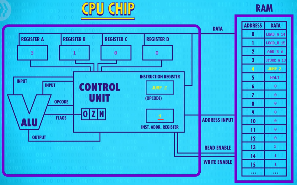
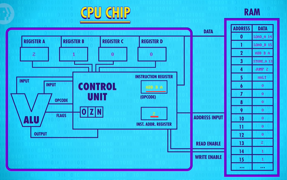
   This causes the processor(处理器CPU) to overwrite the value in the instruction address register, which is currently 4 with the new value, 2. Now, on the processors next fetch cycle, we don’t fetch HALT, instead we fetch the instruction at memory location 2 which is ADD B A. Register A contains the value 2 and register B contains the value 1. So 1+2=3, so now Register A has the value 3. We store that into memory. And we’ve hit he JUMP again, back to ADD B A. Every loop, we’re adding one. Its counting up ! But notice there’s no way to ever escape. This is called an infinite loop - a program that runs forever.

   

5. JUMP_NEGATIVE： computers have other types too - like JUMP IF EQUAL and JUMP IF GREATER.

   Like before, the program starts by loading values from memory into registers A and B. In this example, the number 11 gets loaded into Register A, and 5 gets loaded into Register B. Now we subtract register B from register A. Thats 11 minus 5, which is 6, and so 6 gets saved into Register A

   

   Now we hit our JUMP_NEGATIVE. The last ALU result was 6. That’s a positive number, so the negative flag is false. That means the processor does not jump.

   

   So we continue onto the next instruction which is a JUMP 2.

   

   No conditional on this one, so we jump to instruction 2 no matter what.

   

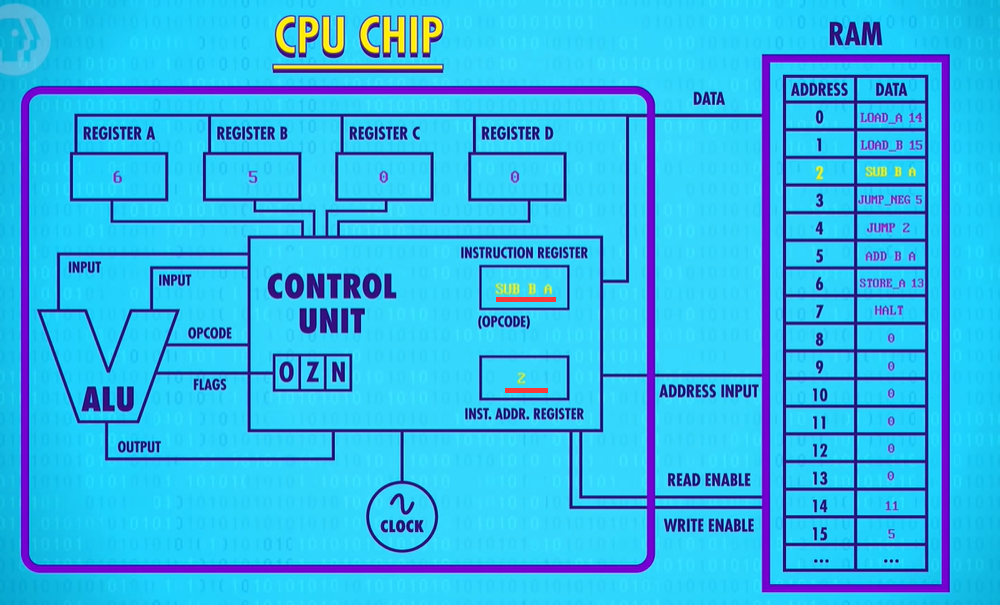
   So we’re back at our SUBTRACT Register B from Register A. 6 minus 5 equals 1. So 1 gets saved into register A. Next instruction. We’re back again at our JUMP_NEGATIVE. 1 is also a positive number, so the CPU continues onto the JUMP 2, looping back around again to the SUBTRACT instruction. This time is different though. 1 minus 5 is negative 4. And so the ALU sets its negative flag to true for the first time.

   

   Now, when we advance to the next instruction, JUMP_NEGATIVE 5 the CPU executes the jump to memory location 5. We’re out of the infinite loop ! Now we have a ADD B to A. Negative 4 plus 5, is positive 1, and we save that into Register A.

   

   Next we have a STORE instruction that saves Register A into memory address 13.

   

   Lastly, we hit our HALT instruction and the computer rests.

   

6. This code calculated the remainder if we divide 5 into 11, which is one.

7. Software also allowed us to do something our hardware could not. Remember, our ALU didn’t have the functionality to divide two numbers, instead it’s the program we made that gave us that functionality.

8. For more memory locations, real, modern CPUs use two strategies

   • The most straightforward approach is just to have bigger instructions, with more bits, like 32 or 64 bits. This is called the instruction length(指令长度).
   • The second approach is to use variable length instructions(可变指令长度). For example, imagine a CPU that uses 8 bit opcodes. When the CPU sees an instruction that needs no extra values, like the HALT instruction, it can just execute it immediately. However, if it sees something like a JUMP instruction, it knows it must also fetch the address to jump to, which is saved immediately behind the JUMP instruction in memory. This is called, logically enough, an Immediate Value(立即值). In such processor designs, instructions can be any number of bytes long, which makes the fetch cycle of the CPU a tad more complicated.

9. Now, our example CPU and instruction set is hypothetical, designed to illustrate key working principles.

10. In 19771 Intel released the 4004 processor. It supported 46 instructions.

11. A modern computer processor, like an Intel Core i7, has thousands of different instructions and instruction variants, ranging from one to fifteen bytes long.

Advanced CPU Designs

1. In the early days of electronic computing, processors were typically made faster by improving the switching time of the transistors inside the chip - the ones that makeup all the logic gates, ALUs and other stuff.

2. So most computer processors today have divide as one of the instructions that the ALU can perform in hardware. Of course, this extra circuitry makes the ALU bigger and more complicated to design, but also more capable - a complexity-for-speed trade-off. For instance, modern computer processors now have special circuits for things like graphics operations, decoding compressed video, and encrypting files all of which are operations that would take many many many clock cycles to perform with standard operations.

3. So instruction sets tend to keep getting larger and larger keeping all the old opcodes around for backwards compatibility.

4. Now, high clock speeds and fancy instruction sets lead to another problem - getting data in and out of the CPU quickly enough.

5. the bottleneck is RAM.

   

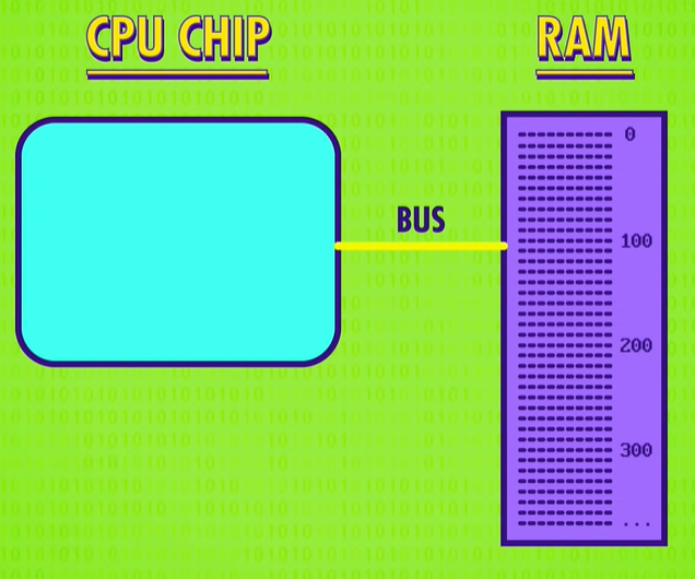
   RAM is typically a memory module that lies outside the CPU. This means that data has to be transmitted to and from RAM along sets of data wires, called a bus(总线). This bus might only be a few centimeters long, and remember those electrical signals are traveling near the speed of light, but when you are operating at gigahertz(千兆赫) speeds – that’s billionths of a second一even this small delay starts to become problematic. It also takes time for RAM itself to lookup the address, retrieve the data and configure itself for output. So a “load from RAM” instruction might take dozens of clock cycles to complete, and during this time the processor is just sitting there idly waiting for the data.

6. One solution is to put a little piece of RAM right on the CPU – called a cache(缓存). There isn’t a lot of space on a processor’s chip so most caches are just kilobytes or maybe megabytes in size, while RAM is usually gigabytes. Having a cache speeds things up in a clever way. When the CPU requests a memory location from RAM, the RAM can transmit not just one single value, but a whole block of data. This takes only a little bit more time, but it allows this data block to be saved into the cache. This tends to be really useful because computer data is often arranged and processed sequentially. Because the cache is so close to the processor, it can typically provide the data in a singled lock cycle – no waiting required.

7. When data requested in RAM is already stored in the cache, it’s called a cache hit(缓存命中), and if the data requested isn’t in the cache, so you have to goto RAM, it’s called a cache miss(缓存未命中).

8. The cache can also be used like a scratch space, storing intermediate values when performing a longer, or more complicated calculation.

9. the cache’s copy of the data is now different to the real version stored in RAM. This mismatch has to be recorded, so that at some point everything can get synced up. For this purpose, the cache has a special flag for each block of memory it stores, called the dirty bit(脏位).

10. Most often this synchronization happens when the cache is full but a new block of memory is being requested by the processor. Before the cache erases the old block to free up space, it checks its dirty bit, and if it’s dirty the old block of data is written back to RAM before loading in the new block.

    

11. Another trick to boost CPU performance is called instruction pipelining(指令流水线).

    Previously, our example processor performed the fetch-decode-execute cycle sequentially and in a continuous loop: Fetch-decode-execute, fetch-decode-execute, fetch-decode-execute, and so on. This meant our design required three clock cycles to execute one instruction.

    

    But each of these stages uses a different part of the CPU, meaning there is an opportunity to parallelize(并行处理) ! While one instruction is getting executed, the next instruction could be getting decoded, and the instruction beyond that fetched from memory. All of these separate processes can overlap so that all parts of the CPU are active at any given time. In this pipelined design, an instruction is executed every single clock cycle which triples the throughput.

    

    But just like with caching, this can lead to some tricky problems. A big hazard is a dependency in the instructions. For example, you might fetch something that the currently executing instruction is just about to modify, which means you’ll end up with the old value in the pipeline. To compensate for this, pipelined processors have to look ahead for data dependencies, and if necessary, stall their pipelines to avoid problems. High end processors, like those found in laptops and smart phones, go one step further and can dynamically reorder instructions with dependencies in order to minimize stalls and keep the pipeline moving, which is called out-of-order execution(乱序执行).

    Another big hazard are conditional jump instructions(条件跳转指令) – we talked about one example, a JUMP NEGATIVE previously. These instructions can change the execution flow of a program depending on a value. A simple pipelined processor will perform a long stall when it sees a jump instruction. Only once the jump outcome is known, does the processor start refilling its pipeline. But, this can produce long delays, so high-end processors have some tricks to deal with this problem too. Imagine an upcoming jump instruction as a fork in a road - a branch. Advanced CPUs guess which way they are going to go, and start filing their pipeline with instructions based off that guess – a technique called speculative execution(推测执行). When the jump instruction is finally resolved, if the CPU guessed correctly, then the pipeline is already full of the correct instructions and it can motor along without delay. However, if the CPU guessed wrong, it has to discard all its speculative results and perform a pipeline flush(清空流水线) . To minimize the effects of these flushes, CPU manufacturers have developed sophisticated ways to guess which way branches will go, called branch prediction(分支预测). Instead of being a 50/50 guess, today’s processors can often guess with over 90% accuracy!

12. In an ideal case, pipelining lets you complete one instruction every single clock cycle, but then superscalar processors(超标量处理器) came along which can execute more than one instruction per clock cycle. During the execute phase even in a pipelined design, whole areas of the processor might be totally idle. For example, while executing an instruction that fetches a value from memory, the ALU is just going to be sitting there, not doing a thing.

    So why not fetch-and- decode several instructions at once, and whenever possible, execute instructions that require different parts of the CPU all at the same time. But we can take this one step further and add duplicate circuitry for popular instructions. For example, many processors will have four, eight or more identical ALUs, so they can execute many mathematical instructions all in parallel !

    

13. the techniques we’ve discussed so far primarily optimize the execution throughput of a single stream of instructions, but another way to increase performance is to run several streams of instructions at once with multi-core processors(多核处理器). You might have heard of dual core or quad core processors. This means there are multiple independent processing units inside of a single CPU chip. In many ways, this is very much like having multiple separate CPUs, but because they’re tightly integrated, they can share some resources, like cache, allowing the cores to work together on shared computations.

    

14. But, when more cores just isn’t enough, you can build computers with multiple independent CPUS! High end computers, like the servers streaming this video from YouTube’s datacenter, often need. the extra horsepower to keep it silky smooth for the hundreds of people watching simultaneously.

15. Two- and four-processor configuration are the most common right now, but every now and again even that much processing power isn’t enough. So we humans get extra ambitious and build ourselves a supercomputer(超级电脑)! When this video was made, the world’s fastest computer was located in The National Supercomputing Center in Wuxi, China. The Sunway Taihu Light contains a brain-melting 40960 CPUs, each with 256 cores! Thats over ten million cores in total and each one of those cores runs at 145 gigahertz. In total, this machine can process 93 Quadrillion – that’s 93 million-billions floating point math operations per second, knows as FLOPS.

Early Programming

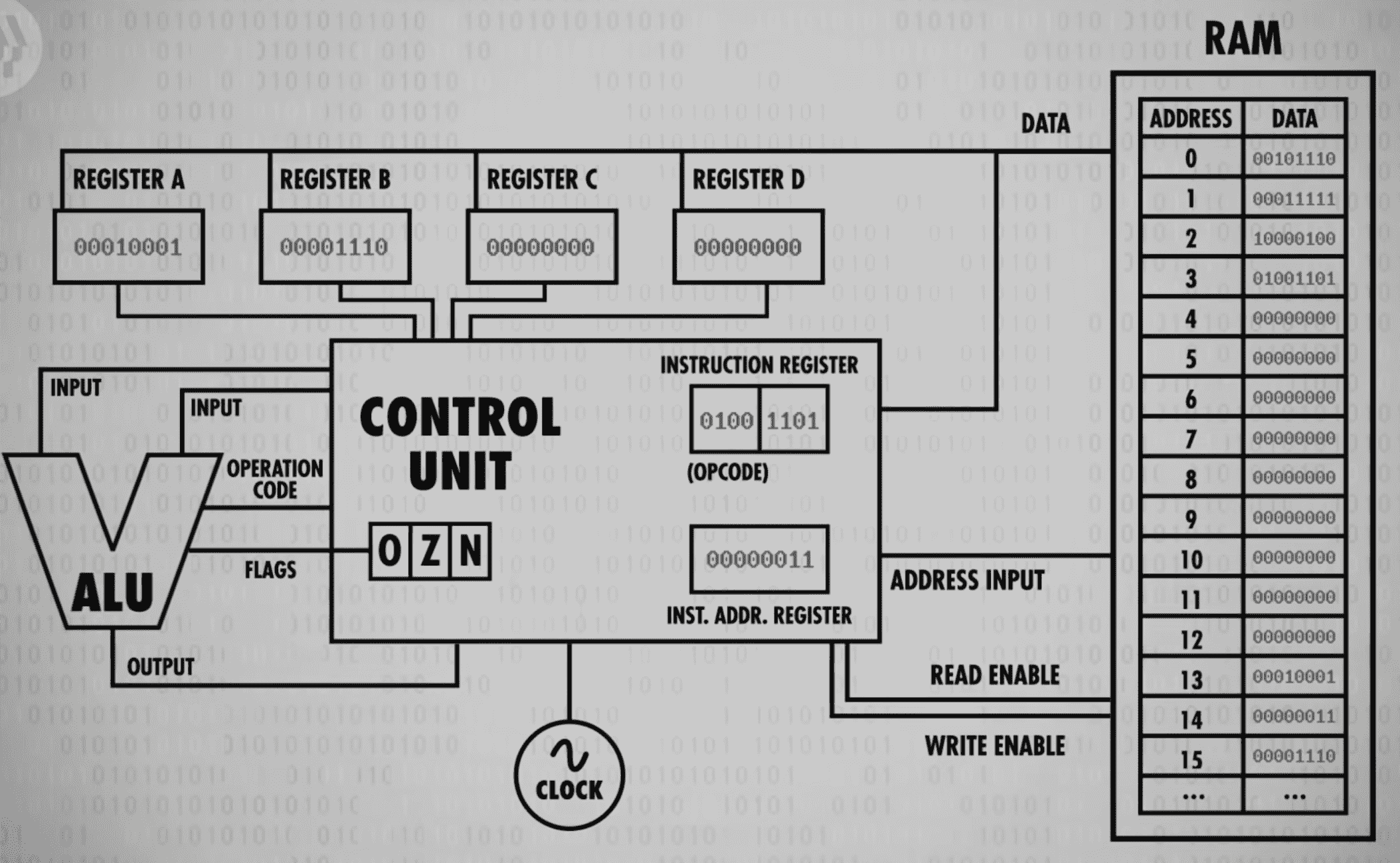
1. in 1801：Joseph Marie Jacquard developed a programmable textile loom. The pattern for each row of the cloth was defined by a punched card(穿孔卡纸). The presence or absence of a hole in the card determined if a specific thread was held high or low in the loom. To vary the pattern across rows these punch cards were arranged in long chains forming a sequence of commands for the loom.

   

2. Nearly a century later, punch cards were used to help tabulate the 1890 US census. Each card held an individual person’s data, things like race, marital status, number of children, country of birth and so on.

   

   For each demographic question a census worker would punch out a hole of the appropriate position. When a card was fed into the tabulating machine, a hole would cause the running total for that specific answer to be increased by one. It is important to note here that early tabulating machines were not truly computers as they can only do one thing-tabulate. Their operation was fixed and not programmable. Over the next 60 years, these business machines grew in capability: add / subtract / multiply / divide and even make simple decisions about when to perform certain operations.

3. To trigger these functions appropriately so that different calculations could be performed, a programmer accessed a control panel(控制面板). This panel was full of little sockets into which a programmer would plug cables to pass values and signals between different parts of the machine for this reason they were also called plug boards(“插线板”).

4. Unfortunately this meant having to rewire the machine each time a different program needed to be run. And so by the 1920s these plug boards were made swappable(可换的). This not only made programming a lot more comfortable but also allowed for different programs be plugged into a machine. For example one board might be wired to calculate sales tax, while another helps with payroll. But plug boards were fiendishly complicated to program.

5. The world’s first general-purpose electronic computer, the ENlAc, completed in 1946, used a ton of plug boards. Even after a program had been completely figured out on paper, physically wiring up the ENlAC and getting the program to run could take upwards of three weeks. Given the enormous cost of these early computers, weeks of downtime simply to switch programs was unacceptable and the new faster more flexible wayto program machines was badly needed. Fortunately by the late 1940s and into the 50s, electronic memory was becoming feasible. As costs fell, memory size grew, instead of storing a program as a physical plug board of wires, it became possible to store a program entirely in a computer’s memory, where it could be easily changed by programmers and quickly accessed by the CPU. These machines were called Stored-program computers(存储程序计算机).

6. With enough computer memory you could store not only the program you wanted to run but also any data your program would need including new values it created along the way. Unifying the program and data into a single shared memory is called the Von Neumann Architecture(“冯诺伊曼结构”). The hallmarks of a Von Neumann computer are a processing unit containing an arithmetic logic unit(计算逻辑单元), data registers(数据寄存器) , instruction register(指令寄存器) , instruction address register(指令地址寄存器) and finally a memory(内存) to store both data and instructions.

   

7. The very first Von Neumann Architecture Stored-program computer was constructed in 1948 by the University of Manchester, nicknamed Baby. And even the computer you are watching this video right now uses the same architecture.

8. Now electronic computer memory is great and all but you still have to load the program and data into the computer before it can run and for this reason punch cards(穿孔纸卡) were used. Well into the 1980s almost all computers have a punch card reader which could suck in a single punch card at a time and write the contents of the card into the computer’s memory. If you load it in a stackof punch cards, the reader would load them all into memorysequentially as a big block. Once the program and data were in memory, the computer would be told to execute it. Of course even simple computer programs might have hundreds of instructions which meant that programs were stored as stacks of punch cards.

9. A common trick was to draw a diagonal line on the side of the card stack called striping, so you’d have at least some clue how to get it back into the right order.

10. The largest program ever punched into punch cards was the US Air Force’s SAGE ar defense system, completed in 1955. And its peak, the project is said to have employed 20% of the world’s programmers. Its main control program was stored on a whopping 62,500 punch cards which is equivalent to roughly 5 megabytes of data.

11. And punch cards weren’t only useful for getting data into computers but also getting data out of them. At the end of a program results could be written out of computer memory and onto punch cards by punching cards. Then this data could be analyzed by humans or loaded into a second program for additional computation.

12. A close cousin to punch cards was punched paper tape(纸带), which is basically the same idea, but continuous instead of being on individual cards

    

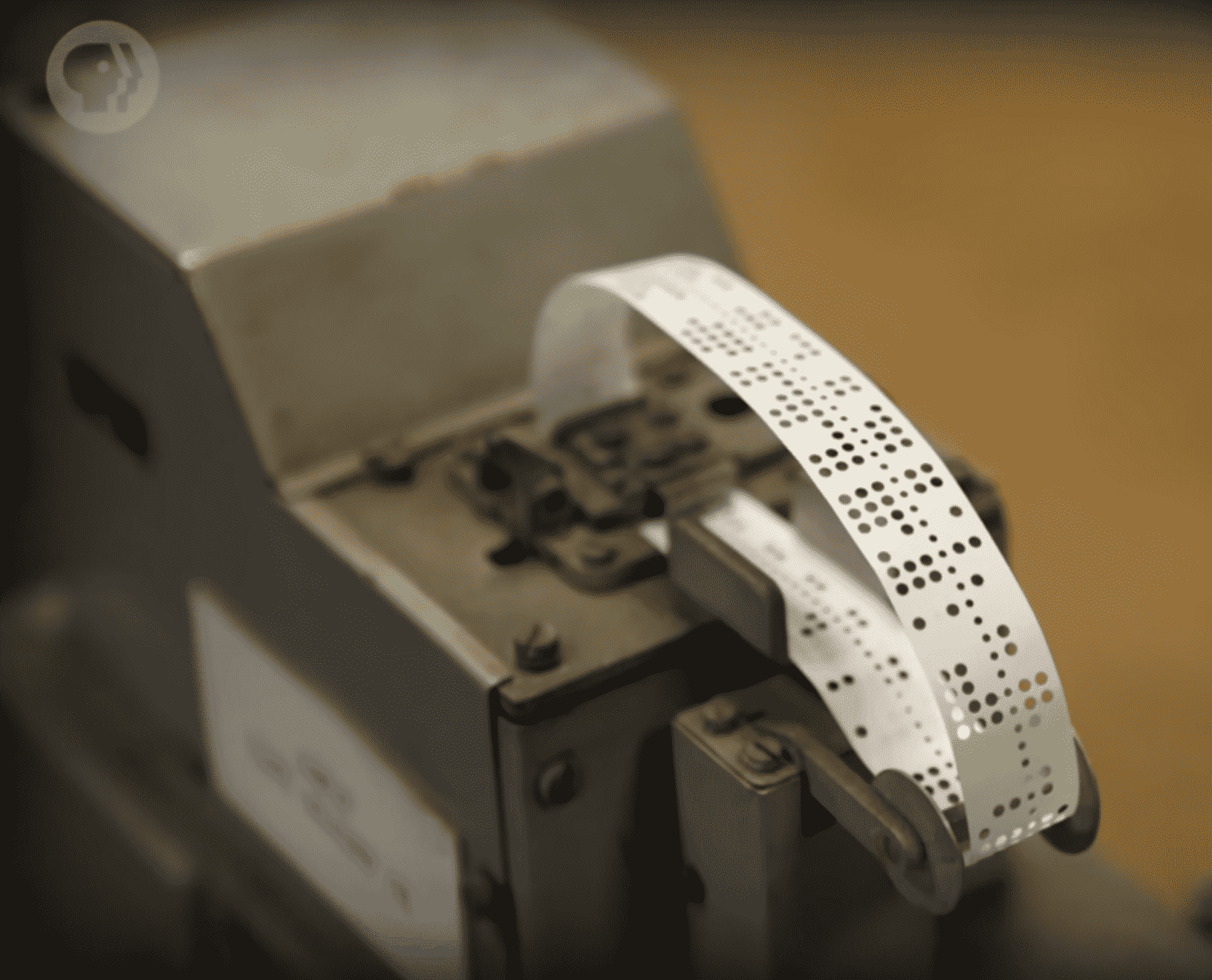
13. Finally in addition to plug boards and punch paper, there was another common way to program and control computers in pre-1980 – Panel programming(面板编程). Rather than having to physically plug in cables to activate certain functions, this could also be done with huge panels full of switches and buttons. And there were indicator lights to display the status of various functions and values in memory. Computers of the 50s and 60s often featured huge control consoles that look like this. Although it was rare to input a whole program using just switches,it was possible.

    

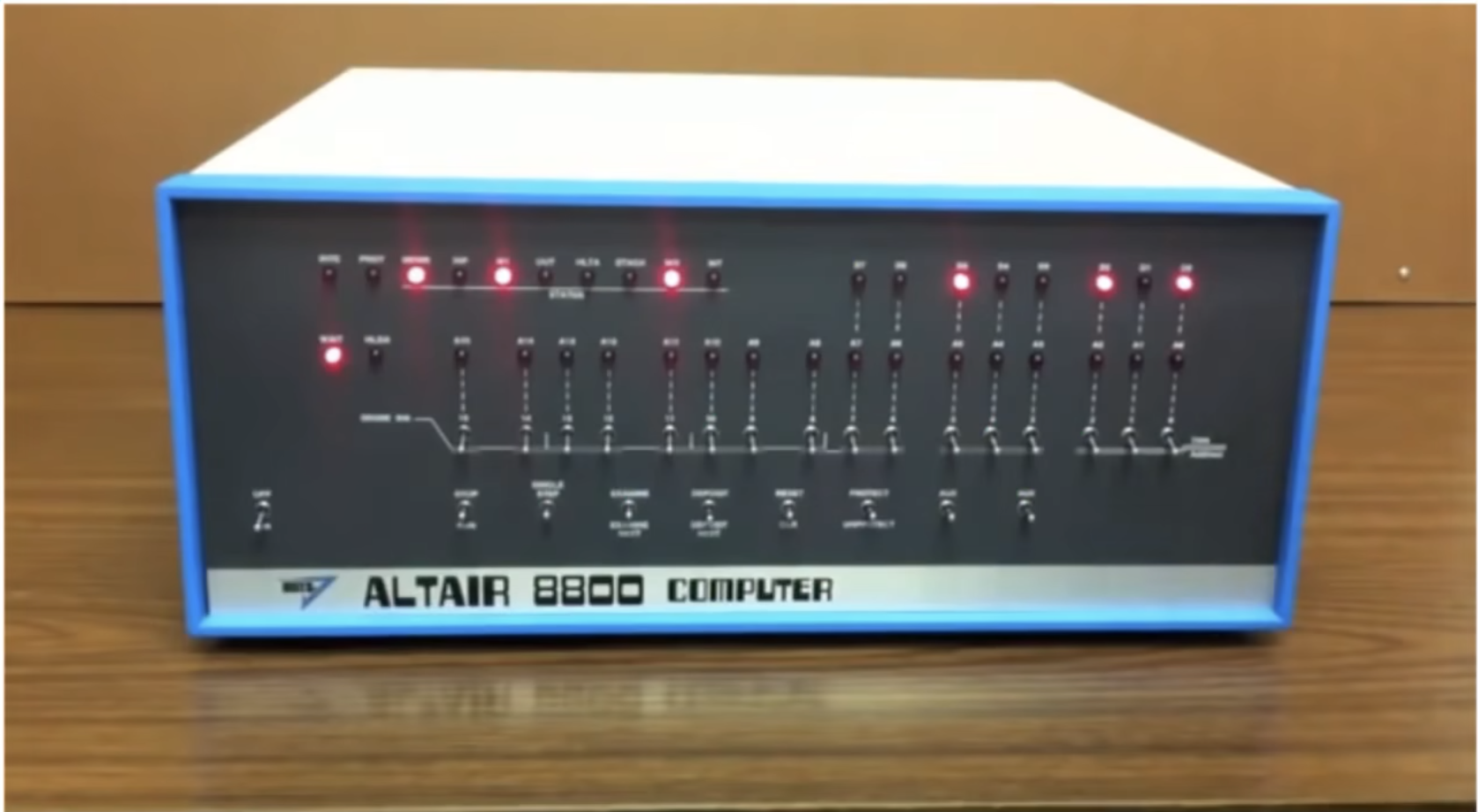
14. And early home computers made for the hobbyist market use switches extensively, because most home users couldn’t afford expensive peripherals like punch card readers. The first commercially successful home computer was the Altair 8800 which sold in two versions: Pre-assembled(预先装好的整税) and the Kit(需要组装的组件).

15. The kit which was popular with amateur computing enthusiasts, sold for the then unprecedented low price are around $400 in 1975.

16. To program the 8800, you’d literally toggle the switches on the front panel to enter the binary op codes for the instruction you wanted. Then you press the deposit button to write that value into memory. Then in the next location in memory you toggle the switches again, for your next instruction deposit it and so on. When you finallyentered yourwhole program into memory, you would toggle the switches moves backto memory address 0, press the run button and watch the little lights blink.

    

17. Whether it was plug board, switches or punched paper, programming these early computers was the realm of experts either professionals who did this for living or technology enthusiasts. You needed intimate knowledge of the underlying hardware, so things like processorop-codes and register wits, to write programs. This meant programming was hard and tedious and even professional engineers and scientists struggled to take full advantage of what computing could offer. What was needed was a simpler way to tell computers what to do.

The First Programming Languages

1. Computer hardware can only handle raw, binary instructions. This is the “language” computer processors natively speak. It’s called Machine Language(机器语言) or Machine Code(机器码).

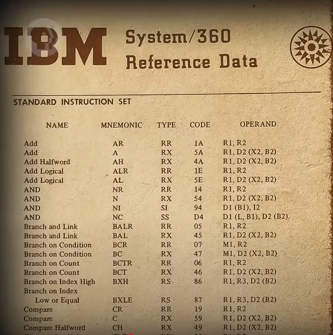
2. In the early days of computing, people had to write entire programs in machine code. More specifically, they’d first write a high-level version of a program on paper, in English. For example “ retrieve the next sale from memory, then add this to the running total for the day, week and year, then calculate any tax to be added” . An informal, high-level description of a program like this is called Pseudo-Code(伪代码). Then, when the program was all figured out on paper, they’d painstakingly expand and translate it into binary, machine code by hand, using things like opcode tables(操作码表). After the translation was complete, the program could be fed into the computer and run.

   

3. By the late 1940s and into the 50s, programmers had developed slightly higher-level languages that were more human-readable. Opcodes were given simple names, called mnemonics(助记符), which were followed by operands(操作数–也就是对应的数据), to form instructions. So instead of having to write instructions as a bunch of 1’s and 0’s, programmers could write something like “LOAD A 14”.

   

   Of course, a CPU has no idea what “LOAD A 14” is. It doesn’t understand text-based language, only binary. And so programmers came up with a clever trick. They created reusable helper programs, in binary, that read in text-based instructions, and assemble them into the corresponding binary instructions automatically. This program is called an Assembler(汇编器). It reads in a program written in an Assembly Language and converts it to native machine code.

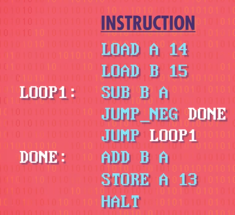
   Over time,Assemblers gained new features that made programming even easier. One nifty feature is automatically figuring out JUMP addresses.

   • Notice how our JUMP NEGATIVE instruction jumps to address 5, and our regular JUMP goes to address 2.

     

   • The problem is, if we add more code to the beginning of this program, all of the addresses would change. That’s a huge pain if you ever want to update your program!

     

   • And so an assembler does away with raw jump addresses, and lets you insert little labels that can be jumped to. When this program is passed into the assembler, it does the work of figuring out all of the jump addresses. Now the programmer can focus more on programming and less on the underlying mechanics under the hood enabling more sophisticated things to be built by hiding unnecessary complexity.

     

4. However, even with nifty assembler features like auto-linking JUMPs to labels, Assembly Languages(汇编语言) are still a thin veneer over machine code. In general, each assembly language instruction converts directly to a corresponding machine instruction - a one-to-one mapping - so it’s inherently tied to the underlying hardware. And the assembler still forces programmers to think about which registers and memory locations they will use. If you suddenly needed an extra value, you might have to change a lot of code to fit it in.

5. This problem did not escape Dr. Grace Hopper(葛丽丝·霍普). As a US naval officer, she was one of the first programmers on the Harvard Mark 1 computer. This was a colossal,electro-mechanical beast. Programs were stored and fed into the computer on punched paper tape(打孔纸带). The Mark 1’s instruction set was so primitive, there weren’t even JUMP instructions. To create code that repeated the same operation multiple times, you’d tape the two ends of the punched tape together, creating a physical loop.

   

   After the war, Hopper continued to work at the forefront of computing. To unleash the potential of computers, she designed a high-level programming language called “Arithmetic Language Version 0(算术语言版本 0)” or A-0 for short. Assembly languages have direct, one-to-one mapping to machine instructions. But a single line of a high-level programming language(高级编程语言) might result in dozens of instructions being executed by the CPU. To perform this complex translation, Hopper built the first compiler(编译器) in 1952. This is a specialized program that transforms “source” code written in a programming language into a low-level language, like assembly or the binary “machine code” that the CPU can directly process.

6. Let’s say we want to add two numbers and save that value. Remember, in assembly code, we had to fetch values from memory, deal with registers, and other low-level details. But this same program can be written in python like so:

   

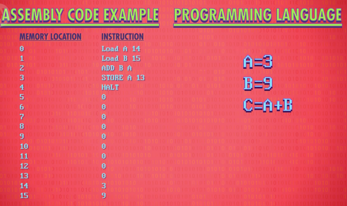
   Notice how there are no registers or memory locations to deal with – the compiler takes care of that stuff, abstracting away a lot of low-level and unnecessary complexity. The programmer just creates abstractions for needed memory locations, known as variables(变量), and gives them names.

7. FORTRAN, derived from “Formula Translation” , was released by IBM a few years later, in 1957, and came to dominate early computer programming. On average, programs written in FORTRAN were 20 times shorter than equivalent handwritten assembly code. Then the FORTRAN Compiler would translate and expand that into native machine code. The community was skeptical that the performance would be as good as hand written code, but the fact that programmers could write more code more quickly, made it an easy choice economically: trading a small increase in computation time for a significant decrease in programmer time. Of course, IBM was in the business of selling computers, and so initially, FORTRAN code could only be compiled and run on IBM computers.

8. And most programing languages and compilers of the 1950s could only run on a single type of computer. So, if you upgraded your computer, you’d often have to re-write all the code too! In response, computer experts from industry, academia and government formed a consortium in 1959 – the Committee on Data Systems languages(数据系统语言委员会), advised by our friend Grace Hopper – to guide the development of a common programming language that could be used across different machines. The result was the high-level, easy to use: Common Business-Oriented Language, or COBOL for short. To deal with different underlying hardware, each computing architecture needed its own COBOL compiler. But critically, these compilers could all accept the same COBOL source code, no matter what computer it was run on. This notion is called write once, run anywhere(一次编写，到处运行). It’s true of most programming languages today.

9. 1960s : ALGOL, LISP and BASIC

10. 1970s : Pascal, C and Smalltalk

11. 1980s : C+ +, Objective-c, and Perl

12. 1990s : python, ruby, and Java

13. the new millennium: Swift, c#, and Go

Programming Basics: Statements & Functions

1. The set of rules that govern the structure and composition of statements in a language is called syntax.

2. A = 5 is a programming language statement. In this case, the statement says a variable named A has the number 5 stored in it. This is called an assignment statement because we’re assigning a value to a variable.

3. Control Flow Statements：

   • An IF statement is like a fork in the road. Which path you take is conditional on whether the expression is true or false – so these expressions are called Conditional Statements.

     • In most programming languages, an if statement looks something like …. “If, expression, then, some code, then end the if statement”.

       IF expression Then 
           code here
           ......
           ......
           END IF
       

     • And If-Statements can be combined with an ELSE statement, which acts as a catch-all if the expression is false.

       IF expression Then 
           code here
           ......
       ELSE
           code here
           ......
           END IF
       

   • To repeat some statements many times, we need to create a conditional loop.

     • One way is a while statement, also called a while loop.

       WHILE expression 
           code to be looped here
           ......
       

     • For Loop：FOR loop is count-controlled; it repeats a specific number of times.

       FOR variable = start_value TO end_value
           code to be looped here
           ......
       NEXT
       

4. To compartmentalize and hide complexity, programming languages can package pieces of code into named functions, also called methods or subroutines in different programming languages.

5. we use a RETURN statement, and specify that the value in ‘result’ be returned.

   FUNCTION exponent(base,)
       result = 1
       FOR: i= 1 TO exp
           RESULT = RESULT X BASE;
       NEXT
   RETURN result
   

6. Modularizing programs into functions not only allows a single programmer to write an entire app, but also allows teams of people to work efficiently on even bigger programs.

7. Modern programming languages come with huge bundles of pre-written functions, called Libraries. These are written by expert coders, made efficient and rigorously tested, and then given to everyone. There are libraries for almost everything, including networking, graphics, and sound.

Robots

1. Robots are machines capable of carrying out a series of actions automatically guided by computer control. How they look isn’t part of the equation. Although the term “robot” is sometimes applied to interactive virtual characters, it’s more appropriate to call these “bots“, or even better, “agents.” That’s because the term “robot“ carries a physical connotation a machine that lives in and acts on the real world.

   “equation” 并不是取其本义 “等式；方程式”，而是一种引申义，表示 “情况；因素；影响因素的总和”。

   connotation /ˌkɒnəˈteɪʃn/ N-COUNT (词或名字的)内涵意义，隐含意义，联想意义

2. The first machines controlled by computers emerged in the late 1940s. These Computer Numerical Control(数控机器) or CNC machines,” could run programs that instructed a machine to perform a series of operations.

3. The first commercial deployment was a programmable industrial robot called the Unimate,sold to General Motors in 1960 to lift hot pieces of metal from a die casting machine and stack them. This was the start of the robotics industry.

   die casting machine /daɪ ˈkɑːstɪŋ məˈʃiːn/ 压铸机

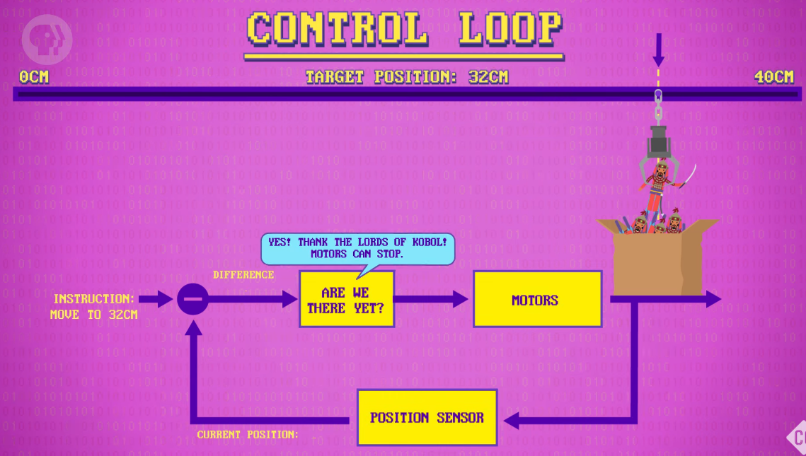
4. a simple control loop（一个简单的控制回路)：

   • First, sense the robot position

   • Are we there yet? Nope. So keep moving.

     

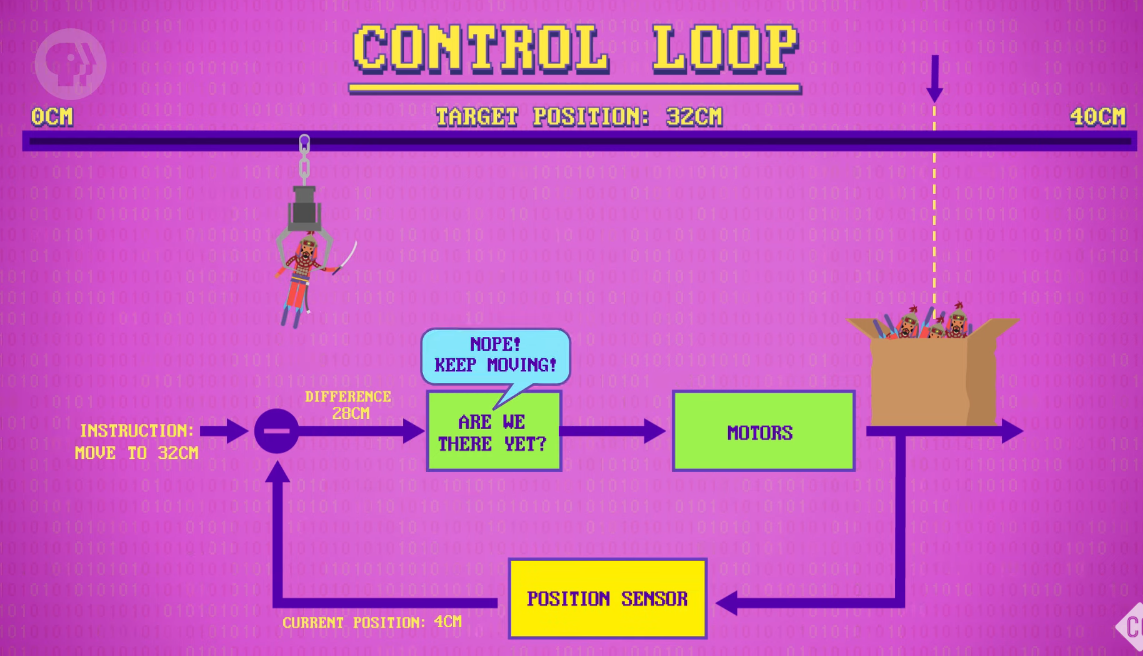
   • Are we there yet? Yes! So we can stop moving.

     

   sense: VERB 感觉到;觉察到;意识到

   Are we there yet 我们到了吗

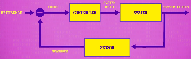
5. a negative feedback loop (负反馈回路)： A negative feedback control loop has three key pieces. There’s a sensor, that measures things in the real world, like water pressure, motor position, air temperature, or whatever you’re trying to control. From this measurement, we calculate how far we are from where we want to be – the error. The error is then interpreted by a controller which decides how to instruct the system to minimize that error. Then, the system acts on the world though pumps, motors, heating elements, and other physical actuators.

   sensor ： 传感器

   controller ： 控制器

   error ： 这里的 error 指的是误差

   interpret ： [ T ] to decide what the intended meaning of something is 理解，解释，阐释

   “acts on the world” 直译为 “对世界产生作用”，在这个句子的语境中，结合 “通过泵、电机、加热元件和其他物理执行器” 这样的描述，更准确的理解是 “与外界环境进行交互并施加影响”

   act on sth （对…）有作用，有影响

   

6. Imagine that our gripper is really heavy and even when the control loop says to stop, momentum causes the gripper to over shoot the desired position. That would cause the control loop to take over again, this time backing the gripper up. A badly tuned control loop might overshoot and overshoot and overshoot, and maybe even wobble forever.

   momentum /məˈmentəm/ N-UNCOUNT (物理学中的)动量，冲量 In physics, momentum is the mass of a moving object multiplied by its speed in a particular direction. 日常生活中可能有人会将 “momentum” 理解为有类似惯性那种 “保持某种趋势” 的感觉，但严格来说在物理学里它们是不同的概念

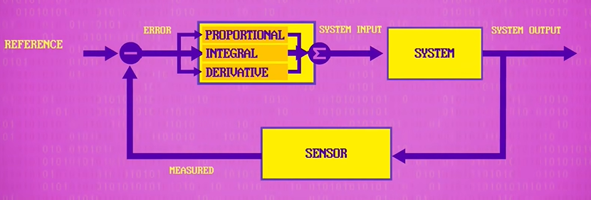
7. proportional-integral-derivative controller（PID controllers） （比例-积分-微分控制器）

   Using the robots speed sensor, we can keep track of its actual speed and plot that alongside its desired speed.

   

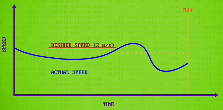
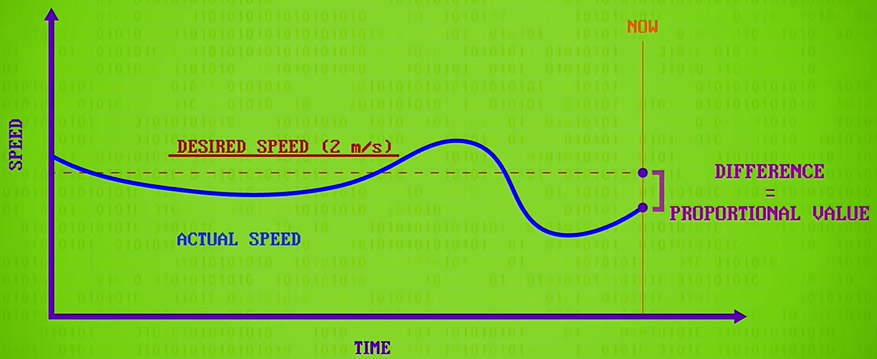
   PID controllers calculate three values from this data. First is the proportional value, which is the difference between the desired value and the actual value at the most recent instant in time or the present. This is what our simpler control loop used before. The bigger the gap between actual and desired, the harder you push towards your target. In other words, it’s proportional control.

   proportional control：比例控制

   

   Next, the integral value is computed, which is the sum of error over a window of time, like the last few seconds. This look-back helps compensate for steady state errors resulting from things like motoring up a long hill. If this value is large, it means proportional control is not enough, and we have to push harder still.

   

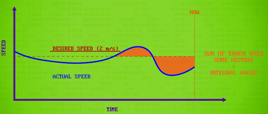
   integral value /ˈɪntɪɡrəl ˈvæljuː/

   • 整数值：指的是整数类型的数值，如 - 2、-1、0、1、2 等，不包含小数或分数部分。比如在数论、离散数学等分支中，经常会讨论变量或表达式取 integral value 的情况。
   • 积分值：在微积分中，是函数在某个区间上积分运算所得到的结果。

   the sum of error ：误差的总和

   look-back: 名词回顾

   look back: 动词回顾

   push harder：①更用力地推 ② 更努力地推进、推动 ③ 更努力尝试

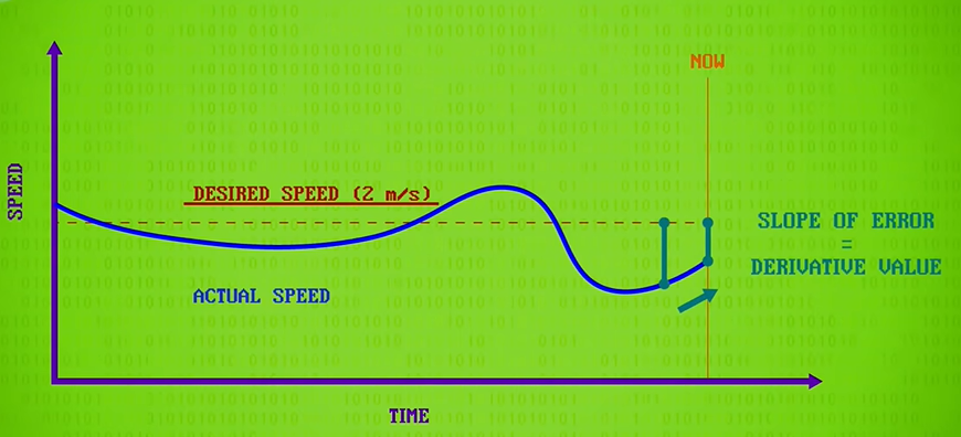
   Finally, there’s the derivative value, which is the rate of change between the desired and actual values. This helps account for possible future error and is sometimes called “anticipatory control“. For example, if you are screaming in towards your goal too fast, you’ll need to ease up a little to prevent overshoot

   

   derivative /dɪˈrɪvətɪv/ ：导数；微商；微分

   anticipatory control 预期控制

   “account for” 常见含义有 “解释；说明；对…… 负责；考虑到” 等，在这个语境中取 “考虑到” 之意

   account for possible future error 考虑到未来可能出现的误差

   These three values are summed together, with different relative weights, to produce a controller output that’s passed to the system.

   weights ：权重

   

8. The danger was obvious to science fiction writer lsaac Asimov(艾萨克·阿西莫夫), who introduced a fictional “Three Laws of Robotics“ in his 1942 shots story Runaround. And then, later he added a zeroth rule.

   • 0 - A robot may not harm humanity, or, by inaction, allow humanity to come to harm.
   • 1 - A robot may not injure a human being or, through inaction, allow a human being to come to harm.
   • 2 - A robot must obey the orders given it by human beings except where such orders would conf lict with the First Law.
   • 3 - A robot must protect its own existence as long as such protection does not conflict with the First or Second Laws.

---

转载请注明来源，欢迎对文章中的引用来源进行考证，欢迎指出任何有错误或不够清晰的表达。可以在下面评论区评论，也可以邮件至 1909773034@qq.com